Climate, oceans and data

Contents

Climate, oceans and data#

Author: Dr. Chelle Gentemann.

This notebook accompanies a lecture for Berkeley’s Data 100 that covers the fundamental physical mechanisms behind global warming and analyzes CO2 and ocean temperature data.

The original resides in this github repository, this is a copy kept as part of the class materials.

Copyright (c) 2021 Chelle Gentemann, MIT Licensed.

import matplotlib.pyplot as plt
import numpy as np
import pandas as pd

# Small style adjustments for more readable plots
plt.style.use("seaborn-whitegrid")
plt.rcParams["figure.figsize"] = (8, 6)
plt.rcParams["font.size"] = 14

/tmp/ipykernel_2149/665068690.py:6: MatplotlibDeprecationWarning: The seaborn styles shipped by Matplotlib are deprecated since 3.6, as they no longer correspond to the styles shipped by seaborn. However, they will remain available as 'seaborn-v0_8-<style>'. Alternatively, directly use the seaborn API instead.
  plt.style.use("seaborn-whitegrid")

Calculate E\(_{in}\) = E\(_{out}\)#

# Solve for T (slide 15)
Ω = 1372  # W/m2 incoming solar
σ = 5.67e-8  # stephan boltzman constant W/m2/K4
A = 0.3
T = ((Ω * (1 - A)) / (4 * σ)) ** 0.25
print("Temperature =", "%.2f" % T, "K")

Temperature = 255.10 K

calculate greenhouse effect#

bonus points for greek letters
to get a sigma type ‘\sigma’ then hit tab

# standard values
Ω = 1372  # W/m2 incoming solar
σ = 5.67e-8  # stephan boltzman constant W/m2/K4
T = 288  # temperature K
E = (T ** 4) * σ - (Ω * (1 - A)) / 4
print("greenhouse effect:", "%.2f" % E, "W m-2")

greenhouse effect: 149.98 W m-2

Experiment#

Solve for the temperature, so that you can see how changes in albedo and greenhouse effect impact T

# Solve for T, including the greenhouse effect
Tnew = (((Ω * (1 - A)) / 4 + E) / σ) ** 0.25
print("temperature =", Tnew, "K")

temperature = 288.0 K

calculate what a change in the greenhouse effect does to temperature#

what if you increase E by 10%

Enew = E * 1.1
Tnew = (((Ω * (1 - 0.3)) / 4 + Enew) / σ) ** 0.25
print("temperature =", "%.2f" % Tnew)
print(
    "10% increase in E leads to ",
    "%.2f" % (Tnew - T),
    " degree K increase in temperature",
)
print(
    "10% increase in E leads to ",
    "%.2f" % (100 * ((Tnew - T) / T)),
    "% increase in temperature",
)

temperature = 290.73
10% increase in E leads to  2.73  degree K increase in temperature
10% increase in E leads to  0.95 % increase in temperature

# read in data and print some

from pathlib import Path

DATA_DIR = Path.home()/Path('shared/climate-data')

monthly_2deg_path = DATA_DIR / "era5_monthly_2deg_aws_v20210920.nc"

file = DATA_DIR / "monthly_in_situ_co2_mlo_cleaned.csv"
data = pd.read_csv(file)
data.head()

	year	month	date_index	fraction_date	c02	data_adjusted_season	data_fit	data_adjusted_seasonally_fit	data_filled	data_adjusted_seasonally_filed
0	1958	1	21200	1958.0411	-99.99	-99.99	-99.99	-99.99	-99.99	-99.99
1	1958	2	21231	1958.1260	-99.99	-99.99	-99.99	-99.99	-99.99	-99.99
2	1958	3	21259	1958.2027	315.70	314.43	316.19	314.90	315.70	314.43
3	1958	4	21290	1958.2877	317.45	315.16	317.30	314.98	317.45	315.16
4	1958	5	21320	1958.3699	317.51	314.71	317.86	315.06	317.51	314.71

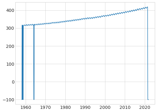
# plot the CO2, note the -99 values you see above showing up in the plot
plt.plot(data["fraction_date"], data["c02"]);

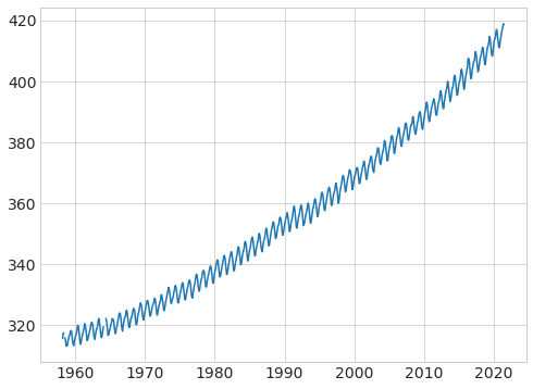
../../_images/e3ed9ab493bda9278787d451b6e89f959f9449b82800f4270514dd5a348e8918.png

# get rid of missing values that are set to -99.99
file = DATA_DIR / "monthly_in_situ_co2_mlo_cleaned.csv"
data = pd.read_csv(file, na_values=-99.99)
data.head()

	year	month	date_index	fraction_date	c02	data_adjusted_season	data_fit	data_adjusted_seasonally_fit	data_filled	data_adjusted_seasonally_filed
0	1958	1	21200	1958.0411	NaN	NaN	NaN	NaN	NaN	NaN
1	1958	2	21231	1958.1260	NaN	NaN	NaN	NaN	NaN	NaN
2	1958	3	21259	1958.2027	315.70	314.43	316.19	314.90	315.70	314.43
3	1958	4	21290	1958.2877	317.45	315.16	317.30	314.98	317.45	315.16
4	1958	5	21320	1958.3699	317.51	314.71	317.86	315.06	317.51	314.71

# plot the data again
plt.plot(data["fraction_date"], data["c02"]);

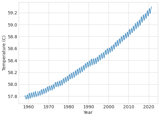
../../_images/0d286c6e98e265f24ab40d6edee1cc3b86b91f5bb01dc307baffad4a27865e0f.png

# use the CO2 in the equation given in class to calculate the greenhouse effect
# then calculate the increase in temperature in deg C rather than K
E = 133.26 + 0.044 * data["c02"]
# calculate new temperature
data["Tnew"] = (((Ω * (1 - 0.3)) / 4 + E) / σ) ** 0.25
plt.plot(data["fraction_date"], (data["Tnew"] - 273.15) * 9 / 5 + 32)
plt.xlabel("Year"), plt.ylabel("Temperature (C)");

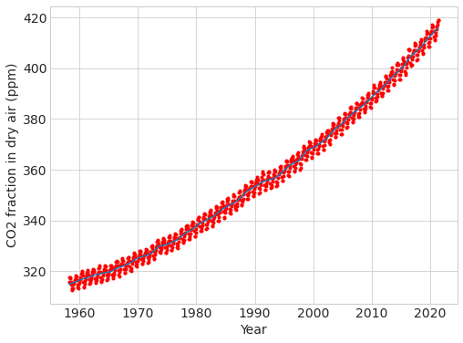
../../_images/372601f371ee435d6753e185bd96a3f58b14f25ebf5370cb3e021e236f8f8204.png

# explore the different data provided in the dataset, what are they?
# can you guess from the names and explain how they were calulated?
# can you re-calculate them? can you re-make the figure in the talk?
plt.plot(data["fraction_date"], data["data_filled"], "r.")
plt.plot(data["fraction_date"], data["data_adjusted_seasonally_fit"])
plt.ylabel("CO2 fraction in dry air (ppm)"), plt.xlabel("Year");

../../_images/55c5642ffb00b26388b0d5fcb5e7c4cd0bf2f6fd1a43e6ae0e5b6579836e2a2a.png

# calculate the annual cycle using groupby
annual = data.groupby(data.month).mean()
annual.head()

	year	date_index	fraction_date	c02	data_adjusted_season	data_fit	data_adjusted_seasonally_fit	data_filled	data_adjusted_seasonally_filed	Tnew
month
1	1989.5	32705.25	1989.541075	356.468571	356.421111	356.461270	356.400952	356.468571	356.421111	287.808514
2	1989.5	32736.25	1989.625925	357.840645	357.139355	357.248889	356.537778	357.240317	356.539841	287.819681
3	1989.5	32764.50	1989.703250	357.965238	356.544603	357.443906	356.010000	357.383750	355.964375	287.820691
4	1989.5	32795.50	1989.788175	359.331270	356.773175	358.718906	356.144844	358.745469	356.190000	287.831802
5	1989.5	32825.50	1989.870325	359.363125	356.253281	359.383750	356.277031	359.363125	356.253281	287.832057

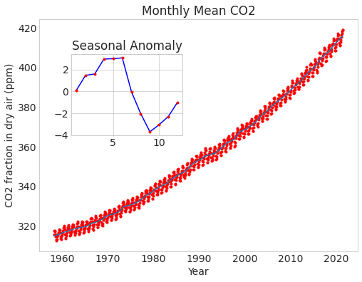
# calculate the anomaly
anomaly = annual - annual.mean()

fig, ax = plt.subplots()

ax.plot("fraction_date", "data_filled", "r.", data=data)
ax.plot("fraction_date", "data_adjusted_seasonally_fit", data=data)
ax.set_xlabel("Year")
ax.set_ylabel("CO2 fraction in dry air (ppm)")
ax.set_title("Monthly Mean CO2")
ax.grid(False)

axin1 = ax.inset_axes([0.1, 0.5, 0.35, 0.35])
axin1.plot(anomaly.c02, "b")
axin1.plot(anomaly.c02, "r.")
axin1.set_title("Seasonal Anomaly");

../../_images/e8c02497e0d6cbad09d10356c7ef0c8bcf356ba95d4c831dcf21106a1b48f030.png

# reading the C02 data from the base file rather than the cleaned up one.
file = DATA_DIR / "monthly_in_situ_co2_mlo.csv"
column_names = [
    "year",
    "month",
    "date_index",
    "fraction_date",
    "c02",
    "data_adjusted_season",
    "data_fit",
    "data_adjusted_seasonally_fit",
    "data_filled",
    "data_adjusted_seasonally_filed",
]
data = pd.read_csv(file, header=0, skiprows=56, names=column_names)
data.head()

	year	month	date_index	fraction_date	c02	data_adjusted_season	data_fit	data_adjusted_seasonally_fit	data_filled	data_adjusted_seasonally_filed
0	1958	1	21200	1958.0411	-99.99	-99.99	-99.99	-99.99	-99.99	-99.99
1	1958	2	21231	1958.1260	-99.99	-99.99	-99.99	-99.99	-99.99	-99.99
2	1958	3	21259	1958.2027	315.70	314.43	316.19	314.90	315.70	314.43
3	1958	4	21290	1958.2877	317.45	315.16	317.30	314.98	317.45	315.16
4	1958	5	21320	1958.3699	317.51	314.71	317.86	315.06	317.51	314.71

.isel versus .sel#

.isel is endpoint EXclusive
.sel is endpoint INclusive

temp = ds.air_temperature_at_2_metres
point1 = temp.isel(time=0, latitude=63, longitude=119)
point2 = temp.sel(time="1979-01", latitude=37.125, longitude=238.875)
area1 = temp.isel(time=0, latitude=slice(63, 65), longitude=slice(119, 125))
area2 = temp.sel(
    time="1979-01",
    latitude=slice(temp.latitude[63], temp.latitude[65]),
    longitude=slice(temp.longitude[119], temp.longitude[125]),
)

print("area1 uses isel")
# print(area1.dims)
print(area1.latitude.data)
print(area1.longitude.data)

area1 uses isel
[37.125 39.125]
[238.875 240.875 242.875 244.875 246.875 248.875]

print("area2 uses sel")
# print(area2.dims)
print(area2.latitude.data)
print(area2.longitude.data)

area2 uses sel
[37.125 39.125 41.125]
[238.875 240.875 242.875 244.875 246.875 248.875 250.875]

point = ds.sel(time="1979-01", latitude=37.125, longitude=238.875)
area = ds.sel(
    time="1979-01",
    latitude=slice(temp.latitude[63], temp.latitude[65]),
    longitude=slice(temp.longitude[119], temp.longitude[125]),
)

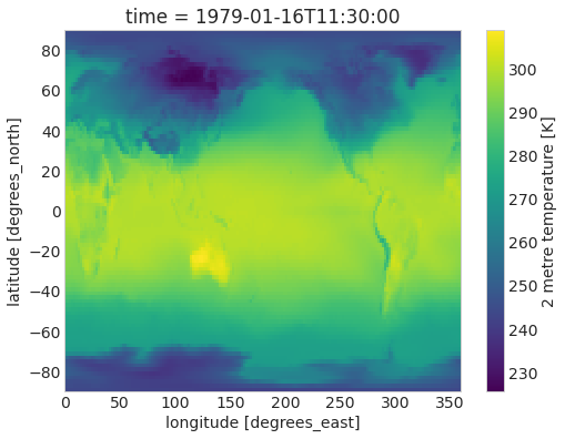
ds.air_temperature_at_2_metres.sel(time="1979-01").plot();

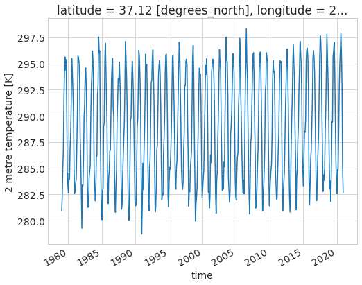
../../_images/35c5b228df95e892caa7d58dc56cb82db0df9f38b7481260c22377e80e4cdc26.png

ds.air_temperature_at_2_metres.sel(latitude=37.125, longitude=238.875).plot();

../../_images/43b16b6e141f9ac7ffb2a6de01acceeeb1ec08ea00fe2da77ead2b9b5174a52b.png

# ds.air_temperature_at_2_metres.mean("time").plot()
mean_map = ds.mean("time")  # takes the mean across all variables in ds
mean_map.air_temperature_at_2_metres.plot();

# calculate a map of the mean values across all time
ave = ds.mean(("latitude", "longitude"))
ave.air_temperature_at_2_metres.plot();

# calculate a map of the mean values across all time
ave = ds.mean("time")
ave.air_temperature_at_2_metres.plot();

# calculate a map of the mean values across all time
ave = ds.mean(("latitude", "longitude"))
ave.air_temperature_at_2_metres.plot();

ave = ds.mean(keep_attrs=True)
ave

weights = np.cos(np.deg2rad(ds.latitude))
weights.name = "weights"
weights.plot();

ds_weighted = ds.weighted(weights)
weighted_mean = ds_weighted.mean()
weighted_mean

ds_weighted = ds.weighted(weights)
weighted_mean = ds_weighted.mean(("latitude", "longitude"))
weighted_mean.air_temperature_at_2_metres.plot();

# calculate the annual cycle
annual_cycle = weighted_mean.groupby("time.month").mean()
annual_cycle.air_temperature_at_2_metres.plot();

# calculate the annual cycle at a point
weighted_trend = (
    weighted_mean.groupby("time.month") - annual_cycle + annual_cycle.mean()
)

weighted_mean.air_temperature_at_2_metres.plot()
weighted_trend.air_temperature_at_2_metres.plot();

bins = np.arange(284, 291, 0.25)
xr.plot.hist(
    weighted_mean.air_temperature_at_2_metres.sel(time=slice("1980", "2000")),
    bins=bins,
    density=True,
    alpha=0.9,
    color="b",
)
xr.plot.hist(
    weighted_mean.air_temperature_at_2_metres.sel(time=slice("2000", "2020")),
    bins=bins,
    density=True,
    alpha=0.85,
    color="r",
)
plt.ylabel("Probability Density (/K)");

pfit = ds.air_temperature_at_2_metres.polyfit("time", 1)
pfit.polyfit_coefficients[0] *= 3.154000000101e16  # go from nanosecond to year
pfit.polyfit_coefficients[0].plot(cbar_kwargs={"label": "trend deg/yr"});

np.timedelta64(1, "Y")
# /np.timedelta64(1,'s').data
pfit.polyfit_coefficients[0, 80, 10] * 3.154000000101e16

import cartopy.crs as ccrs

p = pfit.polyfit_coefficients[0].plot(
    subplot_kws=dict(projection=ccrs.Orthographic(0, 90), facecolor="gray"),
    transform=ccrs.PlateCarree(central_longitude=0),
    cbar_kwargs={"label": "trend deg/yr"},
)

p.axes.coastlines();

Subset all variables to just the Arctic

arctic_ds_weighted = ds.sel(latitude=slice(70,90)).weighted(weights)
arctic_weighted_mean = arctic_ds_weighted.mean(("latitude", "longitude"))
arctic_annual_cycle = arctic_weighted_mean.groupby("time.month").mean()
arctic_weighted_trend = (
    arctic_weighted_mean.groupby("time.month") - arctic_annual_cycle + arctic_annual_cycle.mean()
)

arctic_weighted_mean.air_temperature_at_2_metres.plot()
arctic_weighted_trend.air_temperature_at_2_metres.plot();

def linear_trend(x, y):
    pf = np.polyfit(x, y, 1)
    return pf[0]

x = arctic_weighted_mean.time.dt.year
y = arctic_weighted_mean.air_temperature_at_2_metres
arctic_trend = linear_trend(x, y)
x = weighted_mean.time.dt.year
y = weighted_mean.air_temperature_at_2_metres
trend = linear_trend(x, y)
print('linear trend: global=',trend,'arctic', arctic_trend)

bins = np.arange(245, 280, 1)
xr.plot.hist(
    arctic_weighted_mean.air_temperature_at_2_metres.sel(time=slice("1980", "2000")),
    bins=bins,
    density=True,
    alpha=0.9,
    color="b",
)
xr.plot.hist(
    arctic_weighted_mean.air_temperature_at_2_metres.sel(time=slice("2000", "2020")),
    bins=bins,
    density=True,
    alpha=0.85,
    color="r",
)
plt.ylabel("Probability Density (/K)");