Introduction to Xarray#
In data science setting, it is common to deal with datasets that by nature are tabular and easier to manage. However, how these same ideas translate to designing datasets and datastructures that take into account specific domain knowledge. For example, for earth and climate sciences it is important to manage remote sensing data that usually comes in the form of large dimensional arrays that can include two-dimensional arrays that can contain time series data and measurements in more than one specific band.
Resources:
Acknowledgment: Large part of the contents in this notebook were done by Dr. Chelle Gentemann.
1. Motivation#
Assumptions about how data is structured. For example, the two basic types of datastructures we work in Python are
Lists, matrices, multidimensional arrays: These are very quite common structures in the physical sciences. The main library to manipulate these tensorial structures in Python is
numpy.Tabular data:
pandas, assumption of observations and features This is quite natural datastructures that we often find in data science projects. However, they don’t include all the types of data structures we want to work with.
Note
The library pandas is internally designed using numpy. However, the conceptual setup and the way users manipulate data with the library are radically different.
However, when we start dealing with multidimensional data (eg, three dimensional data involving latitude, longitude and time) we start having problems, including:
how do we keep track of which ones are our coordinate variables? Latitude, longitude and time are quite special physical quantities. If we just work with numpy arrays, we have no way of knowing which dimension corresponds to each coordinate.
How to store multiple datasets using the same coordinate system. Even worse, how do we keep track of datasets with different dimensions? For example, for a dataset that collects temperature measurements, we can imagine using a three dimensional array (lat, lon, time). However, we may want to also include a dataset with surface elevations, for which time is useless and we have a dataset in (lat, lon).
How can we include information in our array about the dataset? This includes the metadata, units, product specifications. Notice that
numpyarrays don’t carry units.
2. Xarray#
import matplotlib.pyplot as plt
import numpy as np
import pandas as pd
#import seaborn as sns
import xarray as xr

#import os
from pathlib import Path

# Small style adjustments for more readable plots
plt.style.use("seaborn-whitegrid")
plt.rcParams["figure.figsize"] = (8, 6)
plt.rcParams["font.size"] = 14
/tmp/ipykernel_386/14117147.py:11: MatplotlibDeprecationWarning: The seaborn styles shipped by Matplotlib are deprecated since 3.6, as they no longer correspond to the styles shipped by seaborn. However, they will remain available as 'seaborn-v0_8-<style>'. Alternatively, directly use the seaborn API instead.
  plt.style.use("seaborn-whitegrid")
For the purposes of this tutorial, we are going to be working with the satellite data product ERA5:
Atmospheric global climate reanalyses
From 1979-2019, hourly estimates of atmospheric, land and oceanic climate variables.
30km global grid with 137 vertical grid points.
Note
Notice where the dataset is stored. If you are running this notebook from the Hub, you will see this is located on our shared folder.
DATA_DIR = Path.home()/Path('shared/climate-data')
monthly_2deg_path = DATA_DIR / "era5_monthly_2deg_aws_v20210920.nc"
ds = xr.open_dataset(monthly_2deg_path)
We can open the .nc dataset directly as a xarray. A xarray.Dataset consists in a collection of objects, including:
Dimensions
Coordinates
Data Variables
You can directly visualize all these objects by displaying the xarray:
ds
<xarray.Dataset>
Dimensions:                                                                                   (
                                                                                               time: 504,
                                                                                               latitude: 90,
                                                                                               longitude: 180)
Coordinates:
  * time                                                                                      (time) datetime64[ns] ...
  * latitude                                                                                  (latitude) float32 ...
  * longitude                                                                                 (longitude) float32 ...
Data variables: (12/15)
    air_pressure_at_mean_sea_level                                                            (time, latitude, longitude) float32 ...
    air_temperature_at_2_metres                                                               (time, latitude, longitude) float32 ...
    air_temperature_at_2_metres_1hour_Maximum                                                 (time, latitude, longitude) float32 ...
    air_temperature_at_2_metres_1hour_Minimum                                                 (time, latitude, longitude) float32 ...
    dew_point_temperature_at_2_metres                                                         (time, latitude, longitude) float32 ...
    eastward_wind_at_100_metres                                                               (time, latitude, longitude) float32 ...
    ...                                                                                        ...
    northward_wind_at_100_metres                                                              (time, latitude, longitude) float32 ...
    northward_wind_at_10_metres                                                               (time, latitude, longitude) float32 ...
    precipitation_amount_1hour_Accumulation                                                   (time, latitude, longitude) float32 ...
    sea_surface_temperature                                                                   (time, latitude, longitude) float32 ...
    snow_density                                                                              (time, latitude, longitude) float32 ...
    surface_air_pressure                                                                      (time, latitude, longitude) float32 ...
Attributes:
    institution:  ECMWF
    source:       Reanalysis
title: ERA5 forecastsThere are a few things we can observe here:
Types of each data object and their respective dimensions.
Metadata
We can observe at the atributes of the datasets by clicking in the icons next to each dataset.
2.1. Basic exploration#
All the datasets can have different contents, but the coordinates are fixed for all of them. In order to access these and their respective name, we can use .dims and .coords:
ds.dims
Frozen({'time': 504, 'latitude': 90, 'longitude': 180})
ds.coords
Coordinates:
  * time       (time) datetime64[ns] 1979-01-16T11:30:00 ... 2020-12-16T11:30:00
  * latitude   (latitude) float32 -88.88 -86.88 -84.88 ... 85.12 87.12 89.12
  * longitude  (longitude) float32 0.875 2.875 4.875 6.875 ... 354.9 356.9 358.9
Just as in pandas, we can read the datasets using two different syntaxes.
temp = ds["air_temperature_at_2_metres"]
temp
<xarray.DataArray 'air_temperature_at_2_metres' (time: 504, latitude: 90,
                                                 longitude: 180)>
[8164800 values with dtype=float32]
Coordinates:
  * time       (time) datetime64[ns] 1979-01-16T11:30:00 ... 2020-12-16T11:30:00
  * latitude   (latitude) float32 -88.88 -86.88 -84.88 ... 85.12 87.12 89.12
  * longitude  (longitude) float32 0.875 2.875 4.875 6.875 ... 354.9 356.9 358.9
Attributes:
    long_name:       2 metre temperature
    nameCDM:         2_metre_temperature_surface
    nameECMWF:       2 metre temperature
    product_type:    analysis
    shortNameECMWF:  2t
    standard_name:   air_temperature
units: Kds.air_temperature_at_2_metres
<xarray.DataArray 'air_temperature_at_2_metres' (time: 504, latitude: 90,
                                                 longitude: 180)>
[8164800 values with dtype=float32]
Coordinates:
  * time       (time) datetime64[ns] 1979-01-16T11:30:00 ... 2020-12-16T11:30:00
  * latitude   (latitude) float32 -88.88 -86.88 -84.88 ... 85.12 87.12 89.12
  * longitude  (longitude) float32 0.875 2.875 4.875 6.875 ... 354.9 356.9 358.9
Attributes:
    long_name:       2 metre temperature
    nameCDM:         2_metre_temperature_surface
    nameECMWF:       2 metre temperature
    product_type:    analysis
    shortNameECMWF:  2t
    standard_name:   air_temperature
units: KNotice that it is easier to keep track of what our code is doing since we can read what the datasets are.
2.2. Subsetting data#
There are three different ways of access subsets of the data
[]: Simple and flexible, but confusing. Also notice we can do this just for DataArrays, while the next ones can be applied directy to the xarray.isel: Integer, positional, end-point exclusing. Still sensitive to error.sel: This is good for labels, end-point inclusive.
In general, when working with thes datasets is better to use sel.
Note
This commands are very similar to the loc and iloc in pandas.
What is the difference between doing slice and then .data or the other wat around?
temp[0, 63, 119].data
array(280.93103, dtype=float32)
temp.data[0, 63, 119]
280.93103
temp.isel(time=0,
          latitude=63,
          longitude=119).data
array(280.93103, dtype=float32)
temp.sel(time="1979-01",
         latitude=37.125,
         longitude=238.875).data
array([280.93103], dtype=float32)
What happens if we want to access the closest point in latitude and longitude? If the key we use for latitude, longitude or time is not in the dataset we will see the following error message:
temp.sel(time="1979-01", latitude=37.126, longitude=238.875)
lat, lon = 37.126, 238.875

abslat = np.abs(ds.latitude - lat)
abslon = np.abs(ds.longitude - lon)

distance2 = abslat ** 2 + abslon ** 2

([xloc, yloc]) = np.where(distance2 == np.min(distance2))

temp.sel(time="1979-01", latitude=ds.latitude.data[xloc], longitude=ds.longitude.data[yloc])
<xarray.DataArray 'air_temperature_at_2_metres' (time: 1, latitude: 1,
                                                 longitude: 1)>
array([[[280.93103]]], dtype=float32)
Coordinates:
  * time       (time) datetime64[ns] 1979-01-16T11:30:00
  * latitude   (latitude) float32 37.12
  * longitude  (longitude) float32 238.9
Attributes:
    long_name:       2 metre temperature
    nameCDM:         2_metre_temperature_surface
    nameECMWF:       2 metre temperature
    product_type:    analysis
    shortNameECMWF:  2t
    standard_name:   air_temperature
units: KWe can also access slices of data
temp.isel(time=0, latitude=slice(63, 65), longitude=slice(119, 125))
<xarray.DataArray 'air_temperature_at_2_metres' (latitude: 2, longitude: 6)>
array([[280.93103, 272.38843, 271.50885, 270.77847, 268.52744, 267.5718 ],
       [276.909  , 268.4416 , 265.8512 , 264.58868, 265.966  , 263.49173]],
      dtype=float32)
Coordinates:
    time       datetime64[ns] 1979-01-16T11:30:00
  * latitude   (latitude) float32 37.12 39.12
  * longitude  (longitude) float32 238.9 240.9 242.9 244.9 246.9 248.9
Attributes:
    long_name:       2 metre temperature
    nameCDM:         2_metre_temperature_surface
    nameECMWF:       2 metre temperature
    product_type:    analysis
    shortNameECMWF:  2t
    standard_name:   air_temperature
units: Ktemp.sel(time="1979-01",
latitude=slice(temp.latitude[63], temp.latitude[65]),
longitude=slice(temp.longitude[119], temp.longitude[125]))
<xarray.DataArray 'air_temperature_at_2_metres' (time: 1, latitude: 3,
                                                 longitude: 7)>
array([[[280.93103, 272.38843, 271.50885, 270.77847, 268.52744, 267.5718 ,
         267.39337],
        [276.909  , 268.4416 , 265.8512 , 264.58868, 265.966  , 263.49173,
         264.07922],
        [269.05563, 266.26437, 265.55194, 263.19815, 264.29312, 261.77335,
         259.54166]]], dtype=float32)
Coordinates:
  * time       (time) datetime64[ns] 1979-01-16T11:30:00
  * latitude   (latitude) float32 37.12 39.12 41.12
  * longitude  (longitude) float32 238.9 240.9 242.9 244.9 246.9 248.9 250.9
Attributes:
    long_name:       2 metre temperature
    nameCDM:         2_metre_temperature_surface
    nameECMWF:       2 metre temperature
    product_type:    analysis
    shortNameECMWF:  2t
    standard_name:   air_temperature
units: K2.3. Making plots#
Making plots with xarray is extremely easy. One of the advantages of using xarray is that the plot will automatically include axis information, since each numerical value in the xarray has assigned a name, either by they coordinate of the dataset product name.
ds.air_temperature_at_2_metres.sel(time="1979-01").plot();
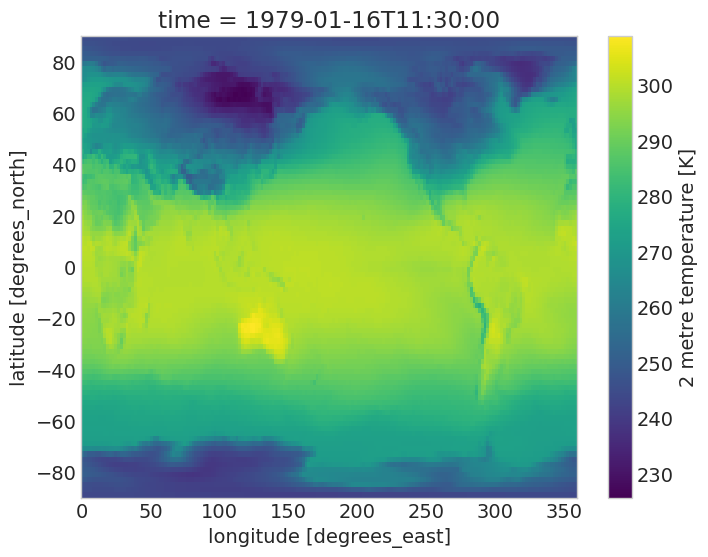
This is just a line of code… quite impressive.
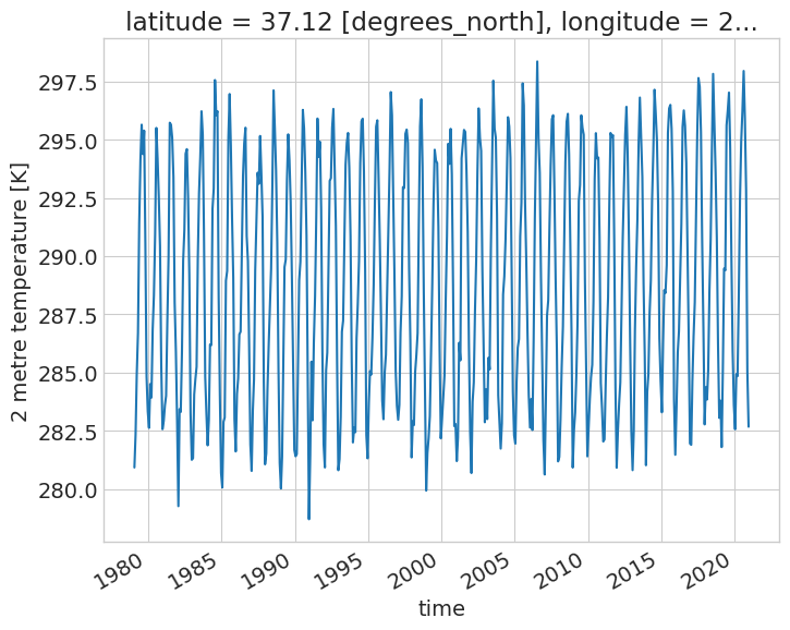
Also, depending what we want to plot, xarray will realize which type of plot we want to make. For example, if we subset in both latitude and longitude, xarray realizes that we want to plot a timeseries:
ds.air_temperature_at_2_metres.sel(latitude=37.125, longitude=238.875).plot();
2.4. Operations with xArray#
In many aspects, you can manipulate xarrays as if you were working with pandas dataframes. For example, you can compute means by
ds.air_temperature_at_2_metres.mean("time")
<xarray.DataArray 'air_temperature_at_2_metres' (latitude: 90, longitude: 180)>
array([[228.23622, 228.2012 , 228.1636 , ..., 228.33353, 228.29826,
        228.26756],
       [228.58359, 228.43468, 228.2972 , ..., 229.14705, 228.94029,
        228.75558],
       [228.8029 , 228.41632, 228.07332, ..., 230.17851, 229.69302,
        229.23451],
       ...,
       [260.34787, 260.42014, 260.47144, ..., 260.13943, 260.22015,
        260.28165],
       [259.83597, 259.8577 , 259.88016, ..., 259.74002, 259.76907,
        259.80435],
       [259.41345, 259.4211 , 259.42905, ..., 259.3969 , 259.4033 ,
        259.40765]], dtype=float32)
Coordinates:
  * latitude   (latitude) float32 -88.88 -86.88 -84.88 ... 85.12 87.12 89.12
* longitude (longitude) float32 0.875 2.875 4.875 6.875 ... 354.9 356.9 358.9ds.mean("time").air_temperature_at_2_metres
<xarray.DataArray 'air_temperature_at_2_metres' (latitude: 90, longitude: 180)>
array([[228.23622, 228.2012 , 228.1636 , ..., 228.33353, 228.29826,
        228.26756],
       [228.58359, 228.43468, 228.2972 , ..., 229.14705, 228.94029,
        228.75558],
       [228.8029 , 228.41632, 228.07332, ..., 230.17851, 229.69302,
        229.23451],
       ...,
       [260.34787, 260.42014, 260.47144, ..., 260.13943, 260.22015,
        260.28165],
       [259.83597, 259.8577 , 259.88016, ..., 259.74002, 259.76907,
        259.80435],
       [259.41345, 259.4211 , 259.42905, ..., 259.3969 , 259.4033 ,
        259.40765]], dtype=float32)
Coordinates:
* latitude (latitude) float32 -88.88 -86.88 -84.88 ... 85.12 87.12 89.12
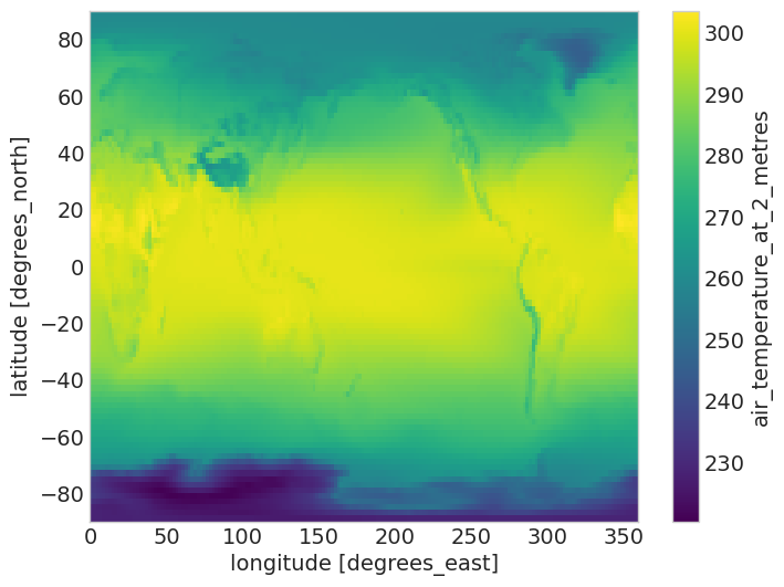
* longitude (longitude) float32 0.875 2.875 4.875 6.875 ... 354.9 356.9 358.9ds.mean("time").air_temperature_at_2_metres.plot()
<matplotlib.collections.QuadMesh at 0x7f88be5ddbd0>
Note
Operations in xarray are lazy: the actual operation you want to perform is not calculated until you really need it.
2.5. Groupby#
Just like you can do it with pandas, you can use groupby with xarray in order to group dataset variables as a function of their coordinates. The most important argument of groupby() is group. When grouping by time attributes, you can use time.dt to access that coordinate as a datetime object.
ds.groupby(ds.time.dt.year).mean()
<xarray.Dataset>
Dimensions:                                                                                   (
                                                                                               year: 42,
                                                                                               latitude: 90,
                                                                                               longitude: 180)
Coordinates:
  * latitude                                                                                  (latitude) float32 ...
  * longitude                                                                                 (longitude) float32 ...
  * year                                                                                      (year) int64 ...
Data variables: (12/15)
    air_pressure_at_mean_sea_level                                                            (year, latitude, longitude) float32 ...
    air_temperature_at_2_metres                                                               (year, latitude, longitude) float32 ...
    air_temperature_at_2_metres_1hour_Maximum                                                 (year, latitude, longitude) float32 ...
    air_temperature_at_2_metres_1hour_Minimum                                                 (year, latitude, longitude) float32 ...
    dew_point_temperature_at_2_metres                                                         (year, latitude, longitude) float32 ...
    eastward_wind_at_100_metres                                                               (year, latitude, longitude) float32 ...
    ...                                                                                        ...
    northward_wind_at_100_metres                                                              (year, latitude, longitude) float32 ...
    northward_wind_at_10_metres                                                               (year, latitude, longitude) float32 ...
    precipitation_amount_1hour_Accumulation                                                   (year, latitude, longitude) float32 ...
    sea_surface_temperature                                                                   (year, latitude, longitude) float32 ...
    snow_density                                                                              (year, latitude, longitude) float32 ...
    surface_air_pressure                                                                      (year, latitude, longitude) float32 ...
Attributes:
    institution:  ECMWF
    source:       Reanalysis
    title:        ERA5 forecasts