Exploratory Data Analysis#
import numpy as np
import pandas as pd
import matplotlib.pyplot as plt
from sklearn.model_selection import train_test_split
import statsmodels.api as sm
import statsmodels.formula.api as smf
from sklearn.metrics import confusion_matrix
from statsmodels.stats.outliers_influence import variance_inflation_factor
from sheltertools.utils import *
import random
import pickle
random.seed(159)
shelter_data = pd.read_csv('./data/Animal_Shelter_Data.csv')
shelter_data.shape
(25008, 24)
shelter_data.head(3)
| Name | Type | Breed | Color | Sex | Size | Date Of Birth | Impound Number | Kennel Number | Animal ID | ... | Intake Subtype | Outcome Type | Outcome Subtype | Intake Condition | Outcome Condition | Intake Jurisdiction | Outcome Jurisdiction | Outcome Zip Code | Location | Count | |
|---|---|---|---|---|---|---|---|---|---|---|---|---|---|---|---|---|---|---|---|---|---|
| 0 | RAZOR | DOG | BOSTON TERRIER | BLACK/WHITE | Neutered | SMALL | 10/29/2009 | K22-043412 | TRUCK | A396382 | ... | FIELD | RETURN TO OWNER | FLD_IDTAG | UNKNOWN | HEALTHY | SANTA ROSA | SANTA ROSA | 95404.0 | 95404(38.43807, -122.71247) | 1 |
| 1 | NaN | OTHER | PIGEON | GRAY/WHITE | Unknown | SMALL | NaN | K23-044095 | TRUCK | A416206 | ... | FIELD | EUTHANIZE | INJ SEVERE | UNKNOWN | HEALTHY | SANTA ROSA | NaN | NaN | NaN | 1 |
| 2 | MAX | DOG | BORDER COLLIE | BLACK/TRICOLOR | Neutered | MED | 03/10/2020 | K23-044090 | DS80 | A399488 | ... | FIELD | RETURN TO OWNER | OVER THE COUNTER_CALL | UNKNOWN | PENDING | COUNTY | COUNTY | 95472.0 | 95472(38.40179, -122.82512) | 1 |
3 rows × 24 columns
shelter_data.columns
Index(['Name', 'Type', 'Breed', 'Color', 'Sex', 'Size', 'Date Of Birth',
       'Impound Number', 'Kennel Number', 'Animal ID', 'Intake Date',
       'Outcome Date', 'Days in Shelter', 'Intake Type', 'Intake Subtype',
       'Outcome Type', 'Outcome Subtype', 'Intake Condition',
       'Outcome Condition', 'Intake Jurisdiction', 'Outcome Jurisdiction',
       'Outcome Zip Code', 'Location', 'Count'],
      dtype='object')
Data Cleaning#
In this step, we dropped all animals that had a missing size.
shelter_data.dropna(subset=['Size'], inplace=True)
shelter_data.isnull().sum()
Name                    6567
Type                       0
Breed                      0
Color                      0
Sex                        0
Size                       0
Date Of Birth           6206
Impound Number             0
Kennel Number             12
Animal ID                  0
Intake Date                0
Outcome Date             159
Days in Shelter            0
Intake Type                0
Intake Subtype             0
Outcome Type             165
Outcome Subtype          482
Intake Condition           0
Outcome Condition        508
Intake Jurisdiction        0
Outcome Jurisdiction    3508
Outcome Zip Code        3565
Location                3565
Count                      0
dtype: int64
EDA#
Number of Animals in the Shelter by Type#
number_of_animals_by_type is a function we wrote for the sheltertools package. It calculates the number of animals per Intake Type.
animal_types = number_of_animals_by_type(shelter_data)
animal_types
Intake Type      Type
ADOPTION RETURN  DOG        292
                 CAT        116
                 OTHER        4
BORN HERE        CAT         16
                 OTHER        1
CONFISCATE       DOG       1456
                 CAT        245
                 OTHER      197
OS APPT          DOG          1
OWNER SURRENDER  CAT       1595
                 DOG       1414
                 OTHER      143
QUARANTINE       DOG        424
                 OTHER      277
                 CAT        118
STRAY            DOG      10223
                 CAT       6603
                 OTHER     1417
TRANSFER         DOG        258
                 CAT        161
                 OTHER       12
Name: Type, dtype: int64
# write animal_types result to file
with open('computation_results/' + 'animal_types.pickle', 'wb') as f:
    pickle.dump(animal_types, f)
Top Breeds by Animal Type#
Top Cat Breeds#
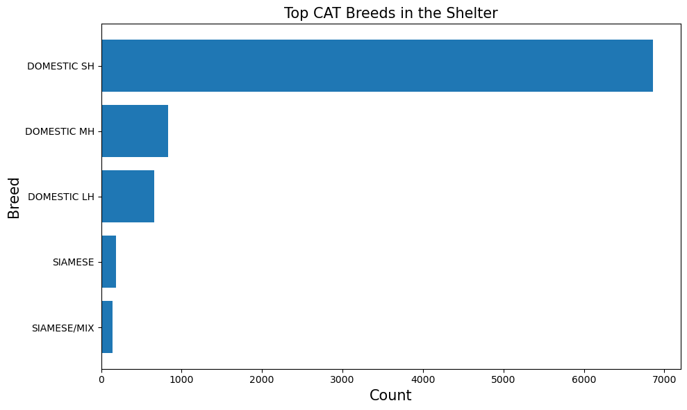
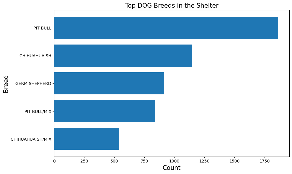
plot_top_breeds is a function we wrote for the sheltertools package. It plots the top breeds for a specified animal type.
plot_top_breeds('CAT', shelter_data)
Top Dog Breeds#
plot_top_breeds('DOG', shelter_data)
Most Common Names#
top_names = shelter_data.groupby(["Type","Name"], as_index=False).size()
top_names = top_names.sort_values(by='size', ascending=False).groupby(["Type"]).head(3)
top_names
| Type | Name | size | |
|---|---|---|---|
| 4614 | DOG | BUDDY | 131 |
| 6004 | DOG | LUNA | 115 |
| 4402 | DOG | BELLA | 104 |
| 2291 | CAT | MILO | 21 |
| 2197 | CAT | LUCY | 19 |
| 758 | CAT | *LUKE | 17 |
| 7727 | OTHER | *JESSICA | 9 |
| 7864 | OTHER | *ROGER | 7 |
| 8036 | OTHER | OREO | 5 |
From the table above, we can see that the top three most common names for dogs at the adoption centers are Buddy, Luna, and Bella. On the other hand, the top three most common names for adopted cats are Milo, Lucy, and Smokey.
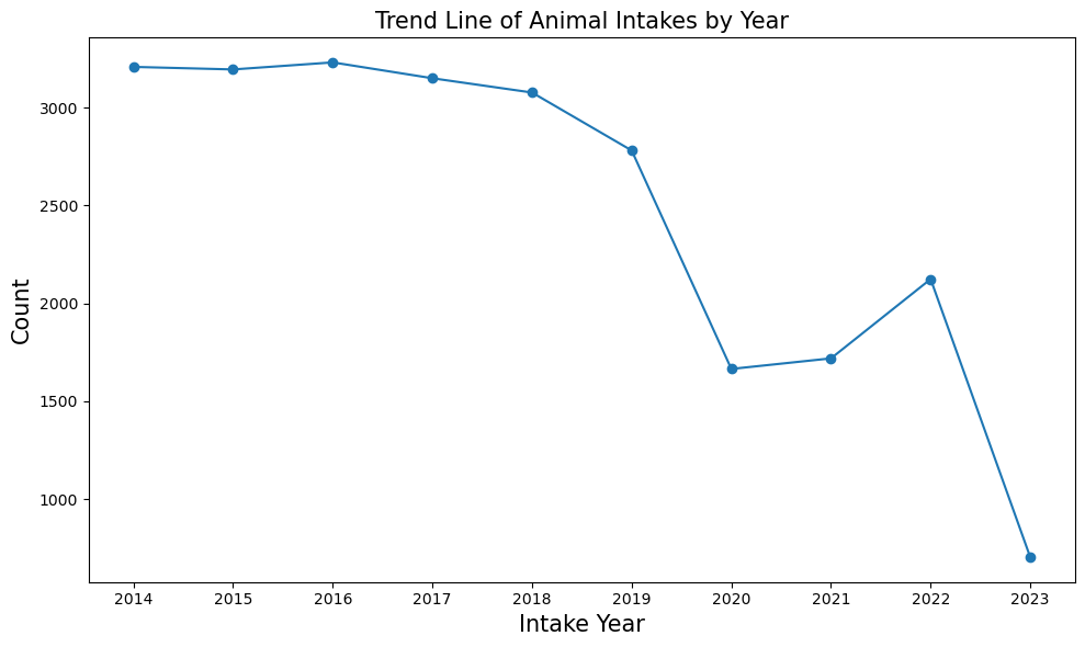
Trend Line: which year has the most number of animal intakes?#
plot_trend_line is a function we wrote for the sheltertools package. It plots the count of animals by year.
plot_trend_line(shelter_data);
Outcomes By Species#
# Select species and outcome type
outcome_data = shelter_data.loc[:,["Type", "Outcome Type"]]
outcome_data
| Type | Outcome Type | |
|---|---|---|
| 0 | DOG | RETURN TO OWNER |
| 1 | OTHER | EUTHANIZE |
| 2 | DOG | RETURN TO OWNER |
| 3 | CAT | DISPOSAL |
| 4 | DOG | TRANSFER |
| ... | ... | ... |
| 25003 | CAT | ADOPTION |
| 25004 | OTHER | TRANSFER |
| 25005 | DOG | EUTHANIZE |
| 25006 | DOG | TRANSFER |
| 25007 | OTHER | RETURN TO OWNER |
24973 rows × 2 columns
# write animal_types result to file
with open('computation_results/' + 'species_outcome.pickle', 'wb') as f:
    pickle.dump(outcome_data, f)
# Drop NA
outcome_data.dropna(subset=['Outcome Type'], inplace=True)
outcome_data.isnull().sum()
Type            0
Outcome Type    0
dtype: int64
# Calculate the proportion of species within each outcome type
top_outcome = outcome_data.groupby([ "Type","Outcome Type"],as_index=False).size()
top_outcome = top_outcome.groupby([ "Type","Outcome Type"], group_keys=False).agg({"size":"sum"}).groupby(
    level=0,group_keys=False).apply(lambda x: 100*x/x.sum()).sort_values(
    by=["Type","size", "Outcome Type"], ascending=[False, False, True])
top_outcome =top_outcome.rename(columns={"size":"percent"})
top_outcome
| percent | ||
|---|---|---|
| Type | Outcome Type | |
| OTHER | TRANSFER | 42.793682 |
| EUTHANIZE | 21.816387 | |
| ADOPTION | 21.273445 | |
| RETURN TO OWNER | 9.871668 | |
| DIED | 2.270484 | |
| DISPOSAL | 1.727542 | |
| ESCAPED/STOLEN | 0.246792 | |
| DOG | RETURN TO OWNER | 50.250609 |
| ADOPTION | 23.600172 | |
| TRANSFER | 14.556781 | |
| EUTHANIZE | 10.826292 | |
| RTOS | 0.264929 | |
| DISPOSAL | 0.250609 | |
| DIED | 0.214807 | |
| ESCAPED/STOLEN | 0.035801 | |
| CAT | ADOPTION | 40.948276 |
| TRANSFER | 26.576679 | |
| EUTHANIZE | 16.254537 | |
| RETURN TO OWNER | 13.214610 | |
| DISPOSAL | 1.780853 | |
| DIED | 1.020871 | |
| RTOS | 0.124773 | |
| ESCAPED/STOLEN | 0.079401 |
# write top outcome result to file
with open('computation_results/' + 'top_outcome.pickle', 'wb') as f:
    pickle.dump(top_outcome, f)
# Create bar plot to visualize most common outcome type within each species
ax = top_outcome.pivot_table(index="Type", columns="Outcome Type").plot(kind='bar')
ax.legend(loc='center left', bbox_to_anchor=(1, 0.5))
ax.set_ylabel("% of Outcome Type")
ax.set_title("Proportion of Outcome Within Each Species");
fig = ax.get_figure()
fig.set_size_inches(8, 6)
fig.savefig('figures/' + 'Proportion_of_Outcome_Within_Each_Species', bbox_inches='tight')
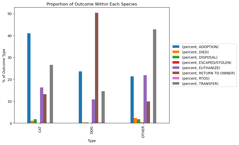
Adoption was the most common outcome for cats at 41%. Half of the dogs in the shelter are being returned to owner, whereas most of the other species (43%) are being transferred.
Shelter Performance#
In this section, we analyze shelter performance based on Adoption rate, Transfer rate, Return-to-owner rate, and Euthanasia Rate.
# Display the overall rates for each species and outcome type throughout all years
rates_df = top_outcome.pivot_table(index="Type", columns="Outcome Type")
rates_df
| percent | ||||||||
|---|---|---|---|---|---|---|---|---|
| Outcome Type | ADOPTION | DIED | DISPOSAL | ESCAPED/STOLEN | EUTHANIZE | RETURN TO OWNER | RTOS | TRANSFER |
| Type | ||||||||
| CAT | 40.948276 | 1.020871 | 1.780853 | 0.079401 | 16.254537 | 13.214610 | 0.124773 | 26.576679 |
| DOG | 23.600172 | 0.214807 | 0.250609 | 0.035801 | 10.826292 | 50.250609 | 0.264929 | 14.556781 |
| OTHER | 21.273445 | 2.270484 | 1.727542 | 0.246792 | 21.816387 | 9.871668 | NaN | 42.793682 |
# write shelter performance result to file
with open('computation_results/' + 'rates_df.pickle', 'wb') as f:
    pickle.dump(rates_df, f)
# Add year column to the dataframe using Outcome Date
outcome_data2 = shelter_data.loc[:,["Outcome Date","Outcome Type"]]
outcome_data2["Outcome Date"] = pd.to_datetime(outcome_data2['Outcome Date'])
outcome_data2["year"] = pd.DatetimeIndex(outcome_data2['Outcome Date']).year
outcome_data2
| Outcome Date | Outcome Type | year | |
|---|---|---|---|
| 0 | 2022-12-26 | RETURN TO OWNER | 2022.0 |
| 1 | 2023-03-15 | EUTHANIZE | 2023.0 |
| 2 | 2023-03-15 | RETURN TO OWNER | 2023.0 |
| 3 | 2022-12-27 | DISPOSAL | 2022.0 |
| 4 | 2023-03-15 | TRANSFER | 2023.0 |
| ... | ... | ... | ... |
| 25003 | 2019-10-23 | ADOPTION | 2019.0 |
| 25004 | 2018-10-10 | TRANSFER | 2018.0 |
| 25005 | 2014-10-02 | EUTHANIZE | 2014.0 |
| 25006 | 2020-08-20 | TRANSFER | 2020.0 |
| 25007 | 2018-03-13 | RETURN TO OWNER | 2018.0 |
24973 rows × 3 columns
# Calculate the proportion of outcome type in each year
yearly_rate = outcome_data2.groupby([ "year","Outcome Type"],as_index=False).size()
yearly_rate = yearly_rate.groupby(["year","Outcome Type"], group_keys=False).agg({"size":"sum"}).groupby(
    level=0,group_keys=False).apply(lambda x: 100*x/x.sum()).sort_values(
    by=["year","size", "Outcome Type"], ascending=[True, False, True]).reset_index()
yearly_rate =yearly_rate.rename(columns={"size":"percent"})
yearly_rate
| year | Outcome Type | percent | |
|---|---|---|---|
| 0 | 2014.0 | ADOPTION | 37.661113 |
| 1 | 2014.0 | RETURN TO OWNER | 33.511474 |
| 2 | 2014.0 | TRANSFER | 14.052185 |
| 3 | 2014.0 | EUTHANIZE | 13.297705 |
| 4 | 2014.0 | DIED | 0.911663 |
| ... | ... | ... | ... |
| 66 | 2023.0 | EUTHANIZE | 13.112392 |
| 67 | 2023.0 | DIED | 1.008646 |
| 68 | 2023.0 | DISPOSAL | 1.008646 |
| 69 | 2023.0 | RTOS | 0.576369 |
| 70 | 2023.0 | ESCAPED/STOLEN | 0.288184 |
71 rows × 3 columns
# Visualize rates
adoption = trend_proportion("ADOPTION", yearly_rate)
euthanize = trend_proportion("EUTHANIZE", yearly_rate)
transferred = trend_proportion("TRANSFER", yearly_rate)
rto = trend_proportion("RETURN TO OWNER", yearly_rate)
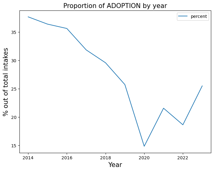
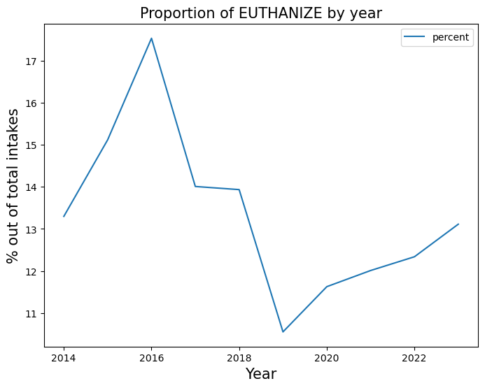
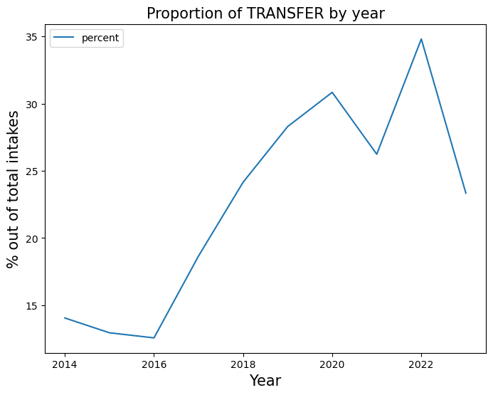
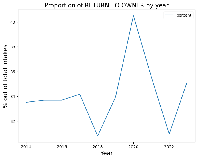
It appears that as the adoption rate declines throughout the years, the shelter chooses to transfer than animals rather than euthanizing.
