
A Comprehensive Analysis Using Machine Learning Techniques#
Introduction#
In this Jupyter Book, we will dive into the world of Airbnb price prediction in Europe. Airbnb has become a popular platform for travelers to find accommodation, offering a wide range of options in various cities across Europe. Understanding the factors that influence pricing is essential for hosts who want to optimize their listings, as well as for guests who want to find the best deals.
Our goal is to build a machine learning model that can predict Airbnb prices based on various features, such as location, room type, amenities, and more. By doing so, we hope to provide valuable insights for both hosts and guests to make informed decisions.
Data Description#
We have a dataset containing Airbnb listings in various European cities, including Amsterdam, Athens, Barcelona, Berlin, Budapest, Lisbon, Paris, Rome, and Vienna. The raw data is from Kaggle, which can be found here.The dataset contains the following features:
City
Price
Day (Weekday or Weekend)
Room Type (Private room, Entire home/apt, Shared room)
Shared Room
Private Room
Person Capacity
Superhost
Multiple Rooms
Business
Cleanliness Rating
Guest Satisfaction
Bedrooms
City Center (km)
Metro Distance (km)
Attraction Index
Normalised Attraction Index
Restaurant Index
Normalised Restaurant Index
Here’s a preview of the dataset:
Import the packages#
import pandas as pd
from IPython.display import Image
from sklearn.model_selection import train_test_split
from utils.pipeline_utils import create_pipelines
Load the data#
df = pd.read_csv('data/Aemf1.csv')
df.head()
| City | Price | Day | Room Type | Shared Room | Private Room | Person Capacity | Superhost | Multiple Rooms | Business | Cleanliness Rating | Guest Satisfaction | Bedrooms | City Center (km) | Metro Distance (km) | Attraction Index | Normalised Attraction Index | Restraunt Index | Normalised Restraunt Index | |
|---|---|---|---|---|---|---|---|---|---|---|---|---|---|---|---|---|---|---|---|
| 0 | Amsterdam | 194.033698 | Weekday | Private room | False | True | 2.0 | False | 1 | 0 | 10.0 | 93.0 | 1 | 5.022964 | 2.539380 | 78.690379 | 4.166708 | 98.253896 | 6.846473 |
| 1 | Amsterdam | 344.245776 | Weekday | Private room | False | True | 4.0 | False | 0 | 0 | 8.0 | 85.0 | 1 | 0.488389 | 0.239404 | 631.176378 | 33.421209 | 837.280757 | 58.342928 |
| 2 | Amsterdam | 264.101422 | Weekday | Private room | False | True | 2.0 | False | 0 | 1 | 9.0 | 87.0 | 1 | 5.748312 | 3.651621 | 75.275877 | 3.985908 | 95.386955 | 6.646700 |
| 3 | Amsterdam | 433.529398 | Weekday | Private room | False | True | 4.0 | False | 0 | 1 | 9.0 | 90.0 | 2 | 0.384862 | 0.439876 | 493.272534 | 26.119108 | 875.033098 | 60.973565 |
| 4 | Amsterdam | 485.552926 | Weekday | Private room | False | True | 2.0 | True | 0 | 0 | 10.0 | 98.0 | 1 | 0.544738 | 0.318693 | 552.830324 | 29.272733 | 815.305740 | 56.811677 |
Exploratory Data Analysis#
Data Preprocessing#
In this section, we performed data preprocessing on the cleaned European Airbnb dataset, which originally had no missing values. We first analyzed the frequency distribution of the prices by plotting a histogram. Upon observing potential outliers in the price distribution, we decided to remove them using the Interquartile Range (IQR) method. By calculating the IQR and determining the lower and upper bounds, we filtered out the outliers from the dataset.
Q1 = df['Price'].quantile(0.25)
Q3 = df['Price'].quantile(0.75)
IQR = Q3 - Q1
lower_bound = Q1 - 1.5 * IQR
upper_bound = Q3 + 1.5 * IQR

filtered_data = df[(df['Price'] >= lower_bound) & (df['Price'] <= upper_bound)]
print(filtered_data.shape)
print(lower_bound)
print(upper_bound)
(38823, 19)
-86.01982524000235
527.4092685023504
Feature Engineering#
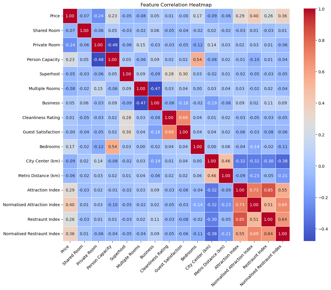
In the Feature Engineering section, we performed various visualizations to better understand the relationships between features and gain insights into the data:
We calculated the correlation matrix to identify potential correlations between variables.
Image(filename = "figures/feature_correlation_heatmap.png")
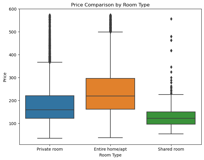
We created a boxplot to compare the price distribution across different room types.
Image(filename = "figures/price_comparison_by_room_type.png")
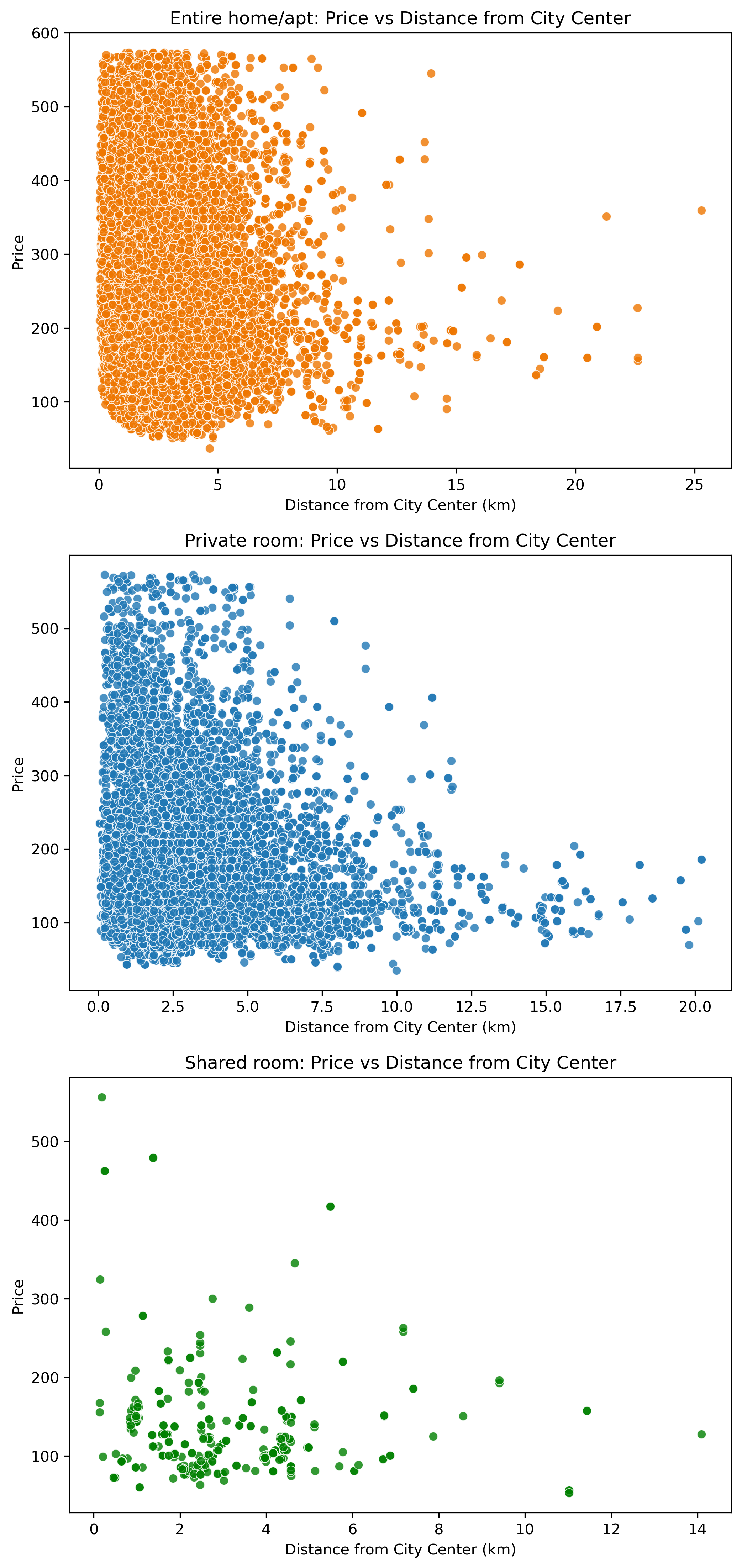
We filtered the data based on room type and generated subplots to visualize the differences between them.
Image(filename = "figures/price_vs_distance_from_city_center_by_room_type.png")
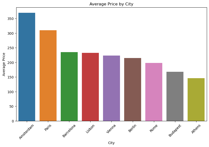
We converted city names to numerical values, which allowed us to better analyze the relationship between the city and price features. We calculated the correlation between city and price is 0.10361768269037437, as well as the average price for each city.
pd.read_csv('results/city_stats.csv')
| City | mean | median | |
|---|---|---|---|
| 0 | Amsterdam | 369.803200 | 368.617158 |
| 1 | Athens | 145.680222 | 127.715417 |
| 2 | Barcelona | 235.001931 | 196.895292 |
| 3 | Berlin | 214.763642 | 185.566047 |
| 4 | Budapest | 168.058828 | 152.277107 |
| 5 | Lisbon | 232.385012 | 223.264540 |
| 6 | Paris | 309.631882 | 289.868580 |
| 7 | Rome | 198.352167 | 182.124237 |
| 8 | Vienna | 223.813612 | 206.624126 |
We created a bar plot to visualize the relationship between city and price, which revealed differences in average prices across cities.
Image(filename = "figures/average_price_by_city.png")
Model Building and Evaluation#
In the Model Building and Evaluation section, various machine learning models are built to predict the price of Airbnb listings. The primary objective is to identify the most effective model for this purpose.
To achieve this, the dataset is first split into training, validation, and testing sets. The training set is used to train the models, the validation set helps tune hyperparameters, and the testing set is employed to evaluate the final model’s performance.
X_train, X_test, y_train, y_test = train_test_split(X, y, test_size=0.2, random_state=1234)
X_train, X_valid, y_train, y_valid = train_test_split(X_train, y_train, test_size=0.2, random_state=331)
The chosen models for this project are Random Forest, Lasso Regression, and Ridge Regression. These models are combined with different imputation methods (Simple Imputer and K-Nearest Neighbors Imputer) to handle any missing values in the data. A total of six combinations are created by pairing each model with an imputation method, and each combination is represented as a pipeline.
create_pipelines()
{'simple_imputer+rf': Pipeline(steps=[('simple_imputer', SimpleImputer(strategy='most_frequent')),
                 ('rf', RandomForestRegressor(min_samples_leaf=5))]),
 'simple_imputer+lasso': Pipeline(steps=[('simple_imputer', SimpleImputer(strategy='most_frequent')),
                 ('lasso', Lasso())]),
 'simple_imputer+ridge': Pipeline(steps=[('simple_imputer', SimpleImputer(strategy='most_frequent')),
                 ('ridge', Ridge())]),
 'knn_imputer+rf': Pipeline(steps=[('knn_imputer', KNNImputer()),
                 ('rf', RandomForestRegressor(min_samples_leaf=5))]),
 'knn_imputer+lasso': Pipeline(steps=[('knn_imputer', KNNImputer()), ('lasso', Lasso())]),
 'knn_imputer+ridge': Pipeline(steps=[('knn_imputer', KNNImputer()), ('ridge', Ridge())])}
Next, we perform an extensive grid search for each pipeline to identify the optimal hyperparameters for each model. The grid search process involves exhaustively trying different combinations of hyperparameters and selecting the combination that yields the best performance. This step is crucial for optimizing the performance of our models, as selecting the appropriate hyperparameters can significantly impact the prediction accuracy and generalization capabilities.
for pipe_name, pipe in pipes.items():

    pipe.fit(X_train, y_train)
cv_param_grid_all = {

    "rf__min_samples_leaf": [1, 3, 5, 10],

    "lasso__alpha": np.logspace(-2, 2, 10),

    "knn_imputer__n_neighbors": [2, 5, 10],

    "ridge__alpha": np.logspace(-3, 7, 10)
}
Once the grid search is completed, and the optimal hyperparameters for each model have been identified, we proceed to evaluate the performance of each pipeline using the validation set. During this step, we make predictions on the validation set and compare these predictions with the actual target values to assess the model’s accuracy.
valid_errs = {}
tuned_pipelines = {}
ypred_valid = {}

for pipe_name, pipe in pipes.items():
    cv_param_grid = {key: cv_param_grid_all[key] for key in cv_param_grid_all.keys() if key.startswith(tuple(pipe.named_steps.keys()))}
    pipe_search = GridSearchCV(pipe, cv_param_grid)
    pipe_search.fit(X_train, y_train)
    valid_errs[pipe_name] = pipe_search.score(X_valid, y_valid)
    tuned_pipelines[pipe_name] = copy.deepcopy(pipe_search)
    ypred_valid[pipe_name] = pipe.predict(X_valid)
To ensure a comprehensive evaluation, we utilize multiple evaluation metrics, including R-squared, Mean Squared Error (MSE), and Mean Absolute Error (MAE). Each of these metrics provides valuable insights into the performance of the models:
R-squared: This metric represents the proportion of the variance in the dependent variable (Price) that can be explained by the independent variables (features) in the model. A higher R-squared value indicates a better fit of the model to the data.
Mean Squared Error (MSE): This metric calculates the average squared difference between the predicted values and the actual values. Lower MSE values indicate better model performance, as the predicted values are closer to the actual values.
Mean Absolute Error (MAE): This metric calculates the average absolute difference between the predicted values and the actual values. Lower MAE values indicate better model performance, as the predicted values are closer to the actual values.
By comparing the results of each pipeline using these evaluation metrics, we can identify the best-performing models and gain valuable insights into their strengths and weaknesses. This comprehensive evaluation allows us to choose the most suitable model for our specific problem and make more accurate predictions on new, unseen
pd.read_csv('results/summary.csv')
| Model | Valid Errors | MSE | MAE | |
|---|---|---|---|---|
| 0 | simple_imputer+rf | 0.741314 | 3423.600482 | 41.317972 |
| 1 | simple_imputer+lasso | 0.574950 | 5854.422403 | 56.484180 |
| 2 | simple_imputer+ridge | 0.574950 | 4861.623952 | 51.632038 |
| 3 | knn_imputer+rf | 0.742253 | 3423.600482 | 41.317972 |
| 4 | knn_imputer+lasso | 0.574950 | 5854.422403 | 56.484180 |
| 5 | knn_imputer+ridge | 0.574950 | 4861.623952 | 51.632038 |
Results and Interpretation#
In this project, various machine learning models were built and evaluated to find the best model for making predictions. The combination of KNN imputer and Random Forest Regressor (knn_imputer+rf) yielded the best performance among the tested models. The evaluation metrics, such as R-squared, Mean Squared Error (MSE), and Mean Absolute Error (MAE), were calculated for the test data. The results indicated that the chosen model provided a good balance between accuracy and interpretability.
pd.read_csv('results/results_df.csv')
| Model | R-squared | MSE | MAE | |
|---|---|---|---|---|
| 0 | knn_imputer+rf | 0.744491 | 2880.713519 | 36.672181 |
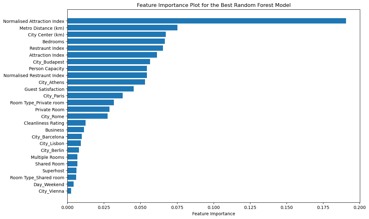
The feature importance analysis further revealed the significant features that contributed the most to the model’s predictions. This information can be utilized to gain valuable insights into the underlying patterns in the data and to guide future decision-making. Overall, the chosen model serves as a reliable tool for making predictions and understanding the relationships between the features and the target variable in the given dataset.
Image(filename = "figures/feature_importance_plot.png")
Conclusion#
This Jupyter Book will take you through the entire process of building a machine learning model to predict Airbnb prices in Europe. You will gain valuable insights into the factors that influence pricing and learn how to leverage these insights to make better decisions as a host or guest.## Conclusion
In this project, we have analyzed the Airbnb Europe dataset, performed data cleaning and preprocessing, and experimented with multiple imputation techniques and regression models to predict the price of Airbnb listings. Our best performing model utilized KNN imputation and a Random Forest regressor, providing satisfactory prediction results.
Through our feature importance analysis, we have identified key factors that influence the price of Airbnb listings. These insights can be beneficial for both hosts and guests when determining appropriate pricing or evaluating listing options.
As a future work, we could explore other advanced machine learning algorithms or ensemble techniques to improve our model’s performance. Additionally, incorporating more data, such as user reviews and historical pricing information, could help enhance our understanding of the factors affecting listing prices and improve the predictive power of our models.
In conclusion, our project provides valuable insights into the Airbnb Europe dataset and demonstrates the potential of data-driven approaches in informing decision-making in the sharing economy.