Data Preprocessing

import pandas as pd
import matplotlib.pyplot as plt
import seaborn as sns

df = pd.read_csv('data/Aemf1.csv')

df.head(10) 

	City	Price	Day	Room Type	Shared Room	Private Room	Person Capacity	Superhost	Multiple Rooms	Business	Cleanliness Rating	Guest Satisfaction	Bedrooms	City Center (km)	Metro Distance (km)	Attraction Index	Normalised Attraction Index	Restraunt Index	Normalised Restraunt Index
0	Amsterdam	194.033698	Weekday	Private room	False	True	2.0	False	1	0	10.0	93.0	1	5.022964	2.539380	78.690379	4.166708	98.253896	6.846473
1	Amsterdam	344.245776	Weekday	Private room	False	True	4.0	False	0	0	8.0	85.0	1	0.488389	0.239404	631.176378	33.421209	837.280757	58.342928
2	Amsterdam	264.101422	Weekday	Private room	False	True	2.0	False	0	1	9.0	87.0	1	5.748312	3.651621	75.275877	3.985908	95.386955	6.646700
3	Amsterdam	433.529398	Weekday	Private room	False	True	4.0	False	0	1	9.0	90.0	2	0.384862	0.439876	493.272534	26.119108	875.033098	60.973565
4	Amsterdam	485.552926	Weekday	Private room	False	True	2.0	True	0	0	10.0	98.0	1	0.544738	0.318693	552.830324	29.272733	815.305740	56.811677
5	Amsterdam	552.808567	Weekday	Private room	False	True	3.0	False	0	0	8.0	100.0	2	2.131420	1.904668	174.788957	9.255191	225.201662	15.692376
6	Amsterdam	215.124317	Weekday	Private room	False	True	2.0	False	0	0	10.0	94.0	1	1.881092	0.729747	200.167652	10.599010	242.765524	16.916251
7	Amsterdam	2771.307384	Weekday	Entire home/apt	False	False	4.0	True	0	0	10.0	100.0	3	1.686807	1.458404	208.808109	11.056528	272.313823	18.975219
8	Amsterdam	1001.804420	Weekday	Entire home/apt	False	False	4.0	False	0	0	9.0	96.0	2	3.719141	1.196112	106.226456	5.624761	133.876202	9.328686
9	Amsterdam	276.521454	Weekday	Private room	False	True	2.0	False	1	0	10.0	88.0	1	3.142361	0.924404	206.252862	10.921226	238.291258	16.604478

Check NAs

df.isna().sum()

City                           0
Price                          0
Day                            0
Room Type                      0
Shared Room                    0
Private Room                   0
Person Capacity                0
Superhost                      0
Multiple Rooms                 0
Business                       0
Cleanliness Rating             0
Guest Satisfaction             0
Bedrooms                       0
City Center (km)               0
Metro Distance (km)            0
Attraction Index               0
Normalised Attraction Index    0
Restraunt Index                0
Normalised Restraunt Index     0
dtype: int64

The dataset we are working with is a cleaned Europe dataset that doesn’t have any missing data (NA values). However, we should still check for any potential outliers that could affect our model’s performance.

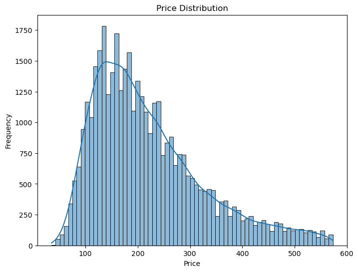
First, let’s plot a histogram to show the frequency distribution of the prices:

# Histogram for price distribution
plt.figure(figsize=(8, 6))
sns.histplot(df['Price'], kde=True)
plt.title('Price Distribution')
plt.xlabel('Price')
plt.ylabel('Frequency')
plt.savefig('figures/price_distribution_before.png', dpi=300, bbox_inches='tight')
plt.show()

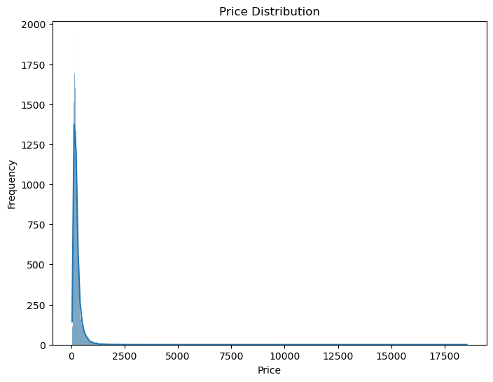
Remove the outliers

From the histogram, we can observe that there seem to be outliers in the price distribution. To address this issue, we will remove the outliers based on the Interquartile Range (IQR) method. Here’s the code to perform this operation:

price_summary = df['Price'].describe()
print(price_summary)
price_summary.to_csv('results/price_summary.csv')

count    41714.000000
mean       260.094423
std        279.408493
min         34.779339
25%        144.016085
50%        203.819274
75%        297.373358
max      18545.450285
Name: Price, dtype: float64

After removing the outliers, we will save the filtered dataset to a filtered CSV file:

# Remove outliers based on Price
Q1 = df['Price'].quantile(0.25)
Q3 = df['Price'].quantile(0.75)
IQR = Q3 - Q1
lower_bound = Q1 - 1.8 * IQR
upper_bound = Q3 + 1.8 * IQR

# Filter out the outliers
filtered_data = df[(df['Price'] >= lower_bound) & (df['Price'] <= upper_bound)]
filtered_data.to_csv('data/filtered_data.csv', index=False)
print(filtered_data.shape)
print(lower_bound)
print(upper_bound)

(39365, 19)
-132.02700727067884
573.4164505330268

# Histogram for price distribution
plt.figure(figsize=(8, 6))
sns.histplot(filtered_data['Price'], kde=True)
plt.title('Price Distribution')
plt.xlabel('Price')
plt.ylabel('Frequency')
plt.savefig('figures/price_distribution.png', dpi=300, bbox_inches='tight')
plt.show()