Analysis Overview

In this project, we aim to answer:

1. Which locations (and even streets, boroughs, and zip codes) in NY have a higher proportion of car accidents?

# !pip install geopandas
# !pip install geoplot

import numpy as np
import pandas as pd
import matplotlib.pyplot as plt
import plotly.express as px
from tool import utils
%matplotlib inline
from datetime import datetime

Importing Data

The dataset we are working with is from the City of New York’s data catalog on motor vehicle crashes. The data contains information from all police reported motor vehicle collisions in NYC in 2012-2023. For the purposes of memory, we only use 2022 data. Click here to download the complete dataset. Be aware that this dataset is quite large and is of 403 Mb.

# read csv into dataframe, specifying the year
crashes = utils.read_csv_of_year(2022)
crashes.head(5)

	Unnamed: 0	CRASH DATE	CRASH TIME	BOROUGH	ZIP CODE	LATITUDE	LONGITUDE	LOCATION	ON STREET NAME	CROSS STREET NAME	...	CONTRIBUTING FACTOR VEHICLE 2	CONTRIBUTING FACTOR VEHICLE 3	CONTRIBUTING FACTOR VEHICLE 4	CONTRIBUTING FACTOR VEHICLE 5	COLLISION_ID	VEHICLE TYPE CODE 1	VEHICLE TYPE CODE 2	VEHICLE TYPE CODE 3	VEHICLE TYPE CODE 4	VEHICLE TYPE CODE 5
0	1	2022-03-26	11:45	NaN	NaN	NaN	NaN	NaN	QUEENSBORO BRIDGE UPPER	NaN	...	NaN	NaN	NaN	NaN	4513547	Sedan	NaN	NaN	NaN	NaN
1	2	2022-06-29	6:55	NaN	NaN	NaN	NaN	NaN	THROGS NECK BRIDGE	NaN	...	Unspecified	NaN	NaN	NaN	4541903	Sedan	Pick-up Truck	NaN	NaN	NaN
2	34	2022-06-29	16:00	NaN	NaN	NaN	NaN	NaN	WILLIAMSBURG BRIDGE OUTER ROADWA	NaN	...	Unspecified	NaN	NaN	NaN	4542336	Motorscooter	Station Wagon/Sport Utility Vehicle	NaN	NaN	NaN
3	37	2022-07-12	17:50	BROOKLYN	11225.0	40.663303	-73.96049	(40.663303, -73.96049)	NaN	NaN	...	Unspecified	NaN	NaN	NaN	4545699	Sedan	NaN	NaN	NaN	NaN
4	38	2022-03-23	10:00	NaN	NaN	NaN	NaN	NaN	NaN	NaN	...	NaN	NaN	NaN	NaN	4512922	Bike	NaN	NaN	NaN	NaN

5 rows × 30 columns

Mapping

Dropping NaNs in Locations column

crashes["LOCATION"].isna().sum()

8938

crashes["LOCATION"].isna().sum()/crashes.shape[0]*100

8.611868538448938

crashes_locations_map = crashes.dropna(subset=["LOCATION"])
# crashes_locations_map.head()

Plotting total casualties

crashes_locations_map["TOTAL CASUALTIES"] = crashes_locations_map["NUMBER OF PERSONS INJURED"] + crashes_locations_map["NUMBER OF PERSONS KILLED"]

/tmp/ipykernel_41499/4161608646.py:1: SettingWithCopyWarning: 
A value is trying to be set on a copy of a slice from a DataFrame.
Try using .loc[row_indexer,col_indexer] = value instead

See the caveats in the documentation: https://pandas.pydata.org/pandas-docs/stable/user_guide/indexing.html#returning-a-view-versus-a-copy
  crashes_locations_map["TOTAL CASUALTIES"] = crashes_locations_map["NUMBER OF PERSONS INJURED"] + crashes_locations_map["NUMBER OF PERSONS KILLED"]

crashes_locations_map_2plus = crashes_locations_map[crashes_locations_map["TOTAL CASUALTIES"] > 2]

fig = px.scatter_mapbox(crashes_locations_map_2plus,
                        lat="LATITUDE",
                        lon="LONGITUDE",
                        color="TOTAL CASUALTIES",
                        size="TOTAL CASUALTIES",
                        zoom=8,
                        height=800,
                        width=1000, color_continuous_scale='thermal')

fig.update_layout(mapbox_style="open-street-map")
fig.show()

Clustering Analysis

features = crashes_locations_map[['LATITUDE', 'LONGITUDE']]
features

	LATITUDE	LONGITUDE
3	40.663303	-73.960490
5	40.607685	-74.138920
6	40.855972	-73.869896
7	40.790276	-73.939600
8	40.642986	-74.016210
...	...	...
103782	0.000000	0.000000
103783	40.877476	-73.836610
103784	40.690180	-73.935600
103785	40.694485	-73.937350
103786	40.687750	-73.790390

94849 rows × 2 columns

from sklearn.cluster import KMeans
# create kmeans model/object
kmeans = KMeans(
    init="random",
    n_clusters=8,
    n_init=10,
    max_iter=300,
    random_state=42
)

# do clustering
kmeans.fit(features)
# save results
labels = kmeans.labels_

# send back into dataframe and display it
crashes_locations_map['cluster'] = labels
# display the number of mamber each clustering
_clusters = crashes_locations_map.groupby('cluster').count()['COLLISION_ID']
# print(_clusters)

/tmp/ipykernel_41499/4122996422.py:2: SettingWithCopyWarning:


A value is trying to be set on a copy of a slice from a DataFrame.
Try using .loc[row_indexer,col_indexer] = value instead

See the caveats in the documentation: https://pandas.pydata.org/pandas-docs/stable/user_guide/indexing.html#returning-a-view-versus-a-copy

fig = px.scatter_mapbox(crashes_locations_map,
                        lat="LATITUDE",
                        lon="LONGITUDE",
                        color="cluster",
                        size="TOTAL CASUALTIES",
                        zoom=8,
                        height=800,
                        width=1000, color_continuous_scale='thermal')

fig.update_layout(mapbox_style="open-street-map")
fig.show()

EDA

Collisions by Geography

# function to add value labels
# credit: GeeksforGeeks
def addlabels(x, y):
    for i in range(len(x)):
        plt.text(i, y[i]*1.01, y[i], ha="center")

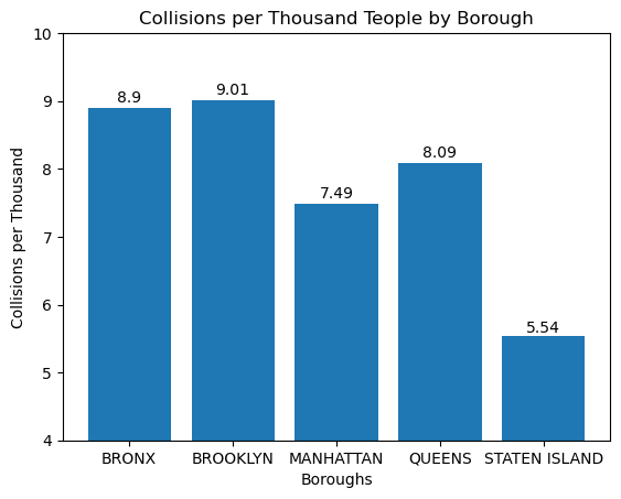
Boroughs

boroughs_data = crashes.groupby("BOROUGH").count()["COLLISION_ID"]

# population source: http://www.citypopulation.de/en/usa/newyorkcity/
population = pd.Series(data={'BRONX': 1379946, 'BROOKLYN': 2590516, 'MANHATTAN': 1596273, 'QUEENS': 2278029, 'STATEN ISLAND': 491133})

per capita

x = boroughs_data.index
y = round(boroughs_data.values / population * 1000, 2)

plt.bar(x, y)
addlabels(x, y)
plt.xlabel("Boroughs")
plt.ylabel("Collisions per Thousand")
plt.title("Collisions per Thousand Teople by Borough")
plt.ylim((4, 10))
plt.savefig("Charts/Collisions per Thousand People by Borough.png")
plt.show()

Zip Code

zc_data = crashes.groupby("ZIP CODE").count()["CRASH DATE"]

zc_df = pd.DataFrame(zc_data).reset_index()
zc_df.rename(columns={"CRASH DATE": "COUNT"}, inplace=True)
zc_df["ZIP CODE"] = zc_df["ZIP CODE"].astype(int)
zc_df.sort_values(by="COUNT", ascending=False)

	ZIP CODE	COUNT
123	11207	1763
128	11212	1128
151	11236	1111
124	11208	1099
119	11203	996
...	...	...
55	10153	1
56	10154	1
58	10158	1
59	10165	1
57	10155	1

210 rows × 2 columns

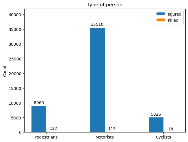
Collisions by Demography

# credit: https://matplotlib.org/stable/gallery/lines_bars_and_markers/barchart.html

types = ("Pedestrians", "Motorists", "Cyclists")
counts = {"Injured": (crashes["NUMBER OF PEDESTRIANS INJURED"].sum(), crashes["NUMBER OF MOTORIST INJURED"].sum(), crashes["NUMBER OF CYCLIST INJURED"].sum()),
          "Killed": (crashes["NUMBER OF PEDESTRIANS KILLED"].sum(), crashes["NUMBER OF MOTORIST KILLED"].sum(), crashes["NUMBER OF CYCLIST KILLED"].sum()),
          }

x = np.arange(len(types))  # the label locations
width = 0.25  # the width of the bars
multiplier = 0

fig, ax = plt.subplots(layout='constrained')

for i, j in counts.items():
    offset = width * multiplier
    rects = ax.bar(x + offset, j, width, label=i)
    ax.bar_label(rects, padding=3)
    multiplier += 1

ax.set_ylabel('Count')
ax.set_title('Type of person')
ax.set_xticks(x + width*0.5, types)
ax.legend()
ax.set_ylim(0, 42000)
plt.savefig("Charts/Collisons by Vehicle")
plt.show()

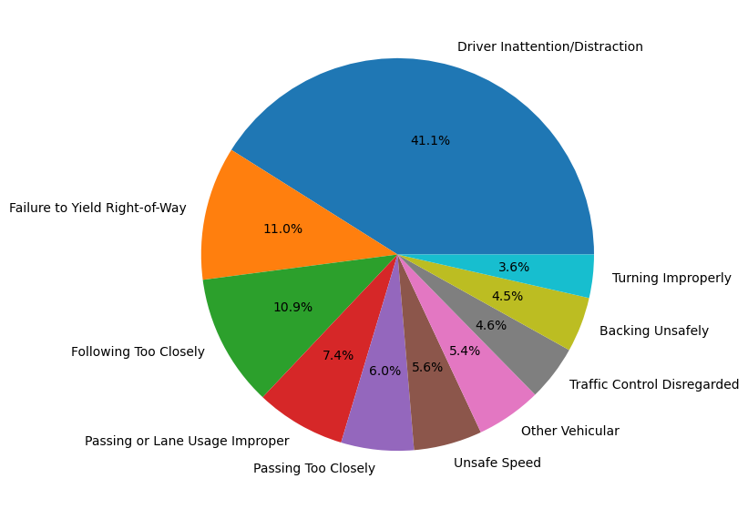
Collisions by Causes

Top 10 Contributing Factor Vehicle 1

cfv = utils.get_contributing_factor(crashes).sort_values("CRASH DATE", ascending=False).iloc[1:11]
labels = cfv.index
sizes = cfv["CRASH DATE"]
fig, ax = plt.subplots(figsize=(10, 7))
ax.pie(sizes, labels=labels, autopct='%1.1f%%')
# plt.legend(labels, bbox_to_anchor=(1.5, 0.25, 0.5, 0.5))
plt.savefig("Charts/Collisions by Contributing Factor")
plt.show()

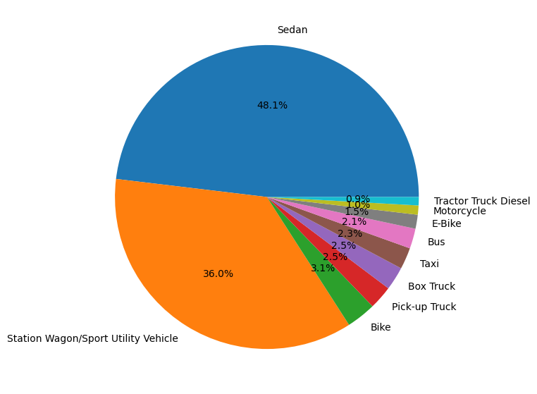
Top 10 Vehicle Type Code 1

# vtc1 = crashes.groupby("VEHICLE TYPE CODE 1").count()["CRASH DATE"].sort_values(ascending=False).head(10)
vtc = utils.get_vehicle_type(crashes).sort_values("CRASH DATE", ascending=False).iloc[:10]
labels = vtc.index
sizes = vtc["CRASH DATE"]

fig, ax = plt.subplots(figsize=(10, 7))
ax.pie(sizes, labels=labels, autopct='%1.1f%%')
plt.savefig("Charts/Collisions by Vehicle Type Code 1")
plt.show()

Collisions by Time

# add month, day and hour to the dataframe
utils.time_processing(crashes)

crashes['CRASH HOUR'][0]

11

crashes

	Unnamed: 0	CRASH DATE	CRASH TIME	BOROUGH	ZIP CODE	LATITUDE	LONGITUDE	LOCATION	ON STREET NAME	CROSS STREET NAME	...	COLLISION_ID	VEHICLE TYPE CODE 1	VEHICLE TYPE CODE 2	VEHICLE TYPE CODE 3	VEHICLE TYPE CODE 4	VEHICLE TYPE CODE 5	CRASH MONTH	CRASH DAY	CRASH HOUR	DAYOFWEEK
0	1	2022-03-26	11:45	NaN	NaN	NaN	NaN	NaN	QUEENSBORO BRIDGE UPPER	NaN	...	4513547	Sedan	NaN	NaN	NaN	NaN	03	26	11	5
1	2	2022-06-29	6:55	NaN	NaN	NaN	NaN	NaN	THROGS NECK BRIDGE	NaN	...	4541903	Sedan	Pick-up Truck	NaN	NaN	NaN	06	29	6	2
2	34	2022-06-29	16:00	NaN	NaN	NaN	NaN	NaN	WILLIAMSBURG BRIDGE OUTER ROADWA	NaN	...	4542336	Motorscooter	Station Wagon/Sport Utility Vehicle	NaN	NaN	NaN	06	29	16	2
3	37	2022-07-12	17:50	BROOKLYN	11225.0	40.663303	-73.96049	(40.663303, -73.96049)	NaN	NaN	...	4545699	Sedan	NaN	NaN	NaN	NaN	07	12	17	1
4	38	2022-03-23	10:00	NaN	NaN	NaN	NaN	NaN	NaN	NaN	...	4512922	Bike	NaN	NaN	NaN	NaN	03	23	10	2
...	...	...	...	...	...	...	...	...	...	...	...	...	...	...	...	...	...	...	...	...	...
103782	1984602	2022-04-24	13:00	BROOKLYN	11233.0	0.000000	0.00000	(0.0, 0.0)	NaN	NaN	...	4621496	Sedan	Station Wagon/Sport Utility Vehicle	Sedan	NaN	NaN	04	24	13	6
103783	1984724	2022-12-06	15:52	BRONX	10475.0	40.877476	-73.83661	(40.877476, -73.83661)	BAYCHESTER AVENUE	GIVAN AVENUE	...	4621506	Sedan	Station Wagon/Sport Utility Vehicle	NaN	NaN	NaN	12	06	15	1
103784	1984763	2022-05-26	0:00	BROOKLYN	11221.0	40.690180	-73.93560	(40.69018, -73.9356)	NaN	NaN	...	4621498	Station Wagon/Sport Utility Vehicle	Station Wagon/Sport Utility Vehicle	NaN	NaN	NaN	05	26	0	3
103785	1984817	2022-07-18	19:00	BROOKLYN	11206.0	40.694485	-73.93735	(40.694485, -73.93735)	LEWIS AVENUE	HART STREET	...	4621495	Bike	NaN	NaN	NaN	NaN	07	18	19	0
103786	1985218	2022-12-11	12:00	QUEENS	11434.0	40.687750	-73.79039	(40.68775, -73.79039)	LINDEN BOULEVARD	157 STREET	...	4622208	Station Wagon/Sport Utility Vehicle	fire truck	NaN	NaN	NaN	12	11	12	6

103787 rows × 34 columns

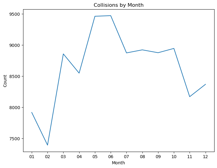
Month

month_data = crashes.groupby("CRASH MONTH").count()["CRASH TIME"]
plt.figure(figsize=(8, 6))
# sns.lineplot(month_data.index, month_data.values)
plt.plot(month_data.index, month_data.values)
plt.title("Collisions by Month")
plt.xlabel("Month")
plt.ylabel("Count")
plt.savefig("Charts/Collisions by Month.png")
plt.show()

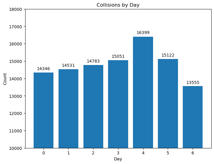
Day

day_data = crashes.groupby("DAYOFWEEK").count()["CRASH TIME"]
plt.figure(figsize=(8, 6))
plt.bar(day_data.index, day_data.values)
addlabels(day_data.index, day_data.values)
plt.title("Collisions by Day")
plt.xlabel("Day")
plt.ylabel("Count")
plt.ylim((10000, 18000))
plt.savefig("Charts/Collisions by Day")
plt.show()

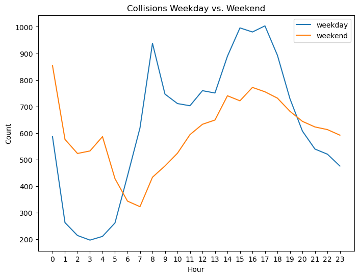
Hour

weekday_hour_data = crashes[crashes['DAYOFWEEK'] < 5].groupby("CRASH HOUR").count()["CRASH TIME"]/5
weekend_hour_data = crashes[crashes['DAYOFWEEK'] > 4].groupby("CRASH HOUR").count()["CRASH TIME"]/2

plt.figure(figsize=(8, 6))
plt.plot(weekday_hour_data.index, weekday_hour_data.values, label='weekday')
plt.plot(weekend_hour_data.index, weekend_hour_data.values, label='weekend')
plt.title("Collisions Weekday vs. Weekend")
plt.xlabel("Hour")
plt.ylabel("Count")
plt.xticks(np.linspace(0, 23, 24))
plt.legend()
plt.savefig("Charts/Collisions Weekday vs. Weekend.png")
plt.show()

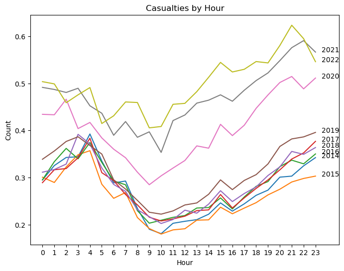
Bivariate analysis:

Investigate relationships between pairs of features, using scatter plots, box plots, or violin plots. For example, you can explore the relationship between contributing factors and the number of persons injured, or between crash time and crash severity.

crashes_18_22 = dict.fromkeys(range(2014, 2023))
for year in crashes_18_22.keys():
    crashes_18_22[year] = utils.read_csv_of_year(year)
    utils.time_processing(crashes_18_22[year])
    α = 1
    crashes_18_22[year]["TOTAL CASUALTIES"] = crashes_18_22[year]["NUMBER OF PERSONS INJURED"] + α * crashes_18_22[year]["NUMBER OF PERSONS KILLED"]

casualties_18_22 = dict.fromkeys(range(2014, 2023))
for year in casualties_18_22.keys():
    casualties_18_22[year] = crashes_18_22[year].groupby("CRASH HOUR")["TOTAL CASUALTIES"].mean()

/home/jovyan/project-group19/tool/utils.py:86: DtypeWarning:

Columns (4) have mixed types. Specify dtype option on import or set low_memory=False.

/home/jovyan/project-group19/tool/utils.py:86: DtypeWarning:

Columns (4) have mixed types. Specify dtype option on import or set low_memory=False.

plt.figure(figsize=(8, 6))
for year in casualties_18_22.keys():
    plt.plot(casualties_18_22[year].index, casualties_18_22[year].values, label=year)
    plt.text(23.5, casualties_18_22[year].values[23], year)
plt.title("Casualties by Hour")
plt.xlabel("Hour")
plt.ylabel("Count")
plt.xticks(np.linspace(0, 23, 24))
plt.xlim((-1, 25))
plt.savefig("Charts/Collisions 2015-2022.png")
plt.show()

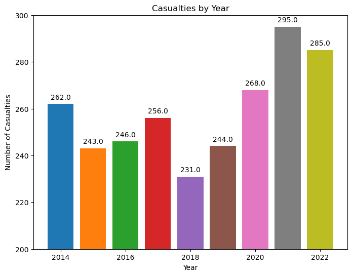
numkilled_18_22 = dict.fromkeys(range(2014, 2023))

for year in crashes_18_22.keys():
    numkilled_18_22[year] = crashes_18_22[year]["NUMBER OF PERSONS KILLED"].sum()

plt.figure(figsize=(8, 6))
for year in casualties_18_22.keys():
    plt.bar(year, numkilled_18_22[year], label=year)
    plt.text(year, numkilled_18_22[year]+2, numkilled_18_22[year], ha="center")
plt.title("Casualties by Year")
plt.xlabel("Year")
plt.ylabel("Number of Casualties")
plt.ylim((200, 300))
plt.savefig("Charts/Plot.png")
plt.show()

Predicting car crash severity

Let’s develop a classification machine learning model using a random forest. Define car accident severity as three levels according to the casualties:

minor injury level: 2 or less people injured, no death reported. Label: 0

major injury level: 3 or more people injured, no death reported. Label: 1

fatal injury level: at least one person killed. Label: 2

injury_conditions = [
    (crashes["NUMBER OF PERSONS KILLED"] >= 1),
    (crashes["NUMBER OF PERSONS INJURED"] >= 3) & (crashes["NUMBER OF PERSONS KILLED"] == 0),
    (crashes["NUMBER OF PERSONS INJURED"] <= 2) & (crashes["NUMBER OF PERSONS KILLED"] == 0),
]

injury_values = [2, 1, 0]

time_conditions = [
    (crashes['CRASH HOUR'] <= 11) & (crashes['CRASH HOUR'] >= 6),
    (crashes['CRASH HOUR'] <= 17) & (crashes['CRASH HOUR'] >= 12),
    (crashes['CRASH HOUR'] <= 5) | (crashes['CRASH HOUR'] >= 18),
]

time_values = ['morning', 'afternoon', 'after sunset']

vehicle1_conditions = [
    (crashes['VEHICLE TYPE CODE 1'].str.contains('Sedan', na=False)),
    (crashes['VEHICLE TYPE CODE 1'].str.contains('Sport', na=False)),
    (crashes['VEHICLE TYPE CODE 1'].str.contains('Truck', na=False)),
    (crashes['VEHICLE TYPE CODE 1'].str.contains('Taxi', na=False)),
    (crashes['VEHICLE TYPE CODE 1'].str.contains('Bus', na=False)),
    (crashes['VEHICLE TYPE CODE 1'].str.contains('Motor', na=False)),
    (crashes['VEHICLE TYPE CODE 1'].str.contains('Bike', na=False)),
    (crashes['VEHICLE TYPE CODE 1'].str.contains('Pick-up', na=False)),
    (crashes['VEHICLE TYPE CODE 1'].notna() | crashes['VEHICLE TYPE CODE 1'].isna())
]
vehicle1_values = ['sedan', 'suv', 'truck', 'taxi', 'bus', 'motor', 'bike', 'pick-up', 'other']

vehicle2_conditions = [
    (crashes['VEHICLE TYPE CODE 2'].str.contains('Sedan', na=False)),
    (crashes['VEHICLE TYPE CODE 2'].str.contains('Sport', na=False)),
    (crashes['VEHICLE TYPE CODE 2'].str.contains('Truck', na=False)),
    (crashes['VEHICLE TYPE CODE 2'].str.contains('Taxi', na=False)),
    (crashes['VEHICLE TYPE CODE 2'].str.contains('Bus', na=False)),
    (crashes['VEHICLE TYPE CODE 2'].str.contains('Motor', na=False)),
    (crashes['VEHICLE TYPE CODE 2'].str.contains('Bike', na=False)),
    (crashes['VEHICLE TYPE CODE 2'].str.contains('Pick-up', na=False)),
    (crashes['VEHICLE TYPE CODE 2'].notna() | crashes['VEHICLE TYPE CODE 2'].isna())
]
vehicle2_values = ['sedan', 'suv', 'truck', 'taxi', 'bus', 'motor', 'bike', 'pick-up', 'other']

# add labels of injury severity
crashes['INJURY LEVEL'] = np.select(injury_conditions, injury_values)
crashes['TIME OF DAY'] = np.select(time_conditions, time_values)
crashes['VEHICLE TYPE 1'] = np.select(vehicle1_conditions, vehicle1_values)
crashes['VEHICLE TYPE 2'] = np.select(vehicle2_conditions, vehicle2_values)

col_list = ['CONTRIBUTING FACTOR VEHICLE 1',
       'CONTRIBUTING FACTOR VEHICLE 2', 'CONTRIBUTING FACTOR VEHICLE 3',
       'CONTRIBUTING FACTOR VEHICLE 4', 'CONTRIBUTING FACTOR VEHICLE 5']
crashes['NUM OF CARS'] = 5 - crashes[col_list].isna().sum(axis=1)

data = crashes[crashes['VEHICLE TYPE 1'] != 'other']
df0 = data[data['INJURY LEVEL'] == 0].sample(20000)
df1 = data[data['INJURY LEVEL'] == 1]
df2 = data[data['INJURY LEVEL'] == 2]
frames = [df0, df1, df2]
data = pd.concat(frames)
data = data.dropna(subset=['BOROUGH'])

features = ['TIME OF DAY', 'NUM OF CARS', 'DAYOFWEEK', 'VEHICLE TYPE 1', 'VEHICLE TYPE 2', 'BOROUGH']  #
X = data[features]
y = data['INJURY LEVEL']

# one hot encoding
encoded_X = pd.get_dummies(X, drop_first=True)
encoded_X

	NUM OF CARS	DAYOFWEEK	TIME OF DAY_afternoon	TIME OF DAY_morning	VEHICLE TYPE 1_bus	VEHICLE TYPE 1_motor	VEHICLE TYPE 1_sedan	VEHICLE TYPE 1_suv	VEHICLE TYPE 1_taxi	VEHICLE TYPE 1_truck	...	VEHICLE TYPE 2_motor	VEHICLE TYPE 2_other	VEHICLE TYPE 2_sedan	VEHICLE TYPE 2_suv	VEHICLE TYPE 2_taxi	VEHICLE TYPE 2_truck	BOROUGH_BROOKLYN	BOROUGH_MANHATTAN	BOROUGH_QUEENS	BOROUGH_STATEN ISLAND
12672	1	0	0	1	0	0	0	0	0	0	...	0	1	0	0	0	0	0	1	0	0
89057	2	0	1	0	0	0	1	0	0	0	...	0	0	1	0	0	0	1	0	0	0
92419	2	1	1	0	0	0	0	1	0	0	...	0	0	0	0	0	1	0	0	1	0
85587	2	5	1	0	0	0	0	1	0	0	...	0	0	0	0	0	0	1	0	0	0
86954	2	3	0	0	0	0	1	0	0	0	...	0	0	1	0	0	0	0	0	1	0
...	...	...	...	...	...	...	...	...	...	...	...	...	...	...	...	...	...	...	...	...	...
103667	1	4	1	0	0	0	0	1	0	0	...	0	1	0	0	0	0	0	1	0	0
103734	1	4	0	0	0	0	0	1	0	0	...	0	1	0	0	0	0	0	0	0	0
103735	2	2	1	0	0	0	0	1	0	0	...	1	0	0	0	0	0	1	0	0	0
103736	2	2	1	0	0	0	0	1	0	0	...	0	0	0	0	0	0	1	0	0	0
103738	1	6	0	0	0	0	0	1	0	0	...	0	1	0	0	0	0	0	1	0	0

14826 rows × 21 columns

run on Random Forest model

# import the necessary liabrary
from sklearn.model_selection import train_test_split
from sklearn.ensemble import RandomForestClassifier
from sklearn.metrics import confusion_matrix, classification_report, f1_score

# train and test split and building baseline model to predict target features
X_train, X_test, y_train, y_test = train_test_split(encoded_X, y, test_size=0.2, random_state=42)

# modelling using random forest baseline
rf = RandomForestClassifier(n_estimators=500, max_depth=30, random_state=42)
rf.fit(X_train, y_train)

# predicting on test data
predics = rf.predict(X_test)

# train score
print('Training accuracy: %.2f %%' % (rf.score(X_train, y_train)*100))
# test score
print('Training accuracy: %.2f %%' % (rf.score(X_test, y_test)*100))

Training accuracy: 91.77 %
Training accuracy: 88.37 %

run on logistic regression model

from sklearn.model_selection import train_test_split
from sklearn.preprocessing import StandardScaler
from sklearn.linear_model import LogisticRegression
from sklearn.pipeline import Pipeline
from sklearn.metrics import roc_curve, roc_auc_score, classification_report, accuracy_score, confusion_matrix 

scaler = StandardScaler()
lr = LogisticRegression()
model1 = Pipeline([('standardize', scaler), ('log_reg', lr)])

model1.fit(X_train, y_train)

Pipeline(steps=[('standardize', StandardScaler()),
                ('log_reg', LogisticRegression())])

In a Jupyter environment, please rerun this cell to show the HTML representation or trust the notebook.
On GitHub, the HTML representation is unable to render, please try loading this page with nbviewer.org.

Pipeline(steps=[('standardize', StandardScaler()),
                ('log_reg', LogisticRegression())])

Pipeline(steps=[('standardize', StandardScaler()),
                ('log_reg', LogisticRegression())])

In a Jupyter environment, please rerun this cell to show the HTML representation or trust the notebook.
On GitHub, the HTML representation is unable to render, please try loading this page with nbviewer.org.

y_train_hat = model1.predict(X_train)
y_train_hat_probs = model1.predict_proba(X_train)[:, 1]
train_accuracy = accuracy_score(y_train, y_train_hat)*100
# print('Confusion matrix:\n', confusion_matrix(y_train, y_train_hat))
print('Training accuracy: %.2f %%' % train_accuracy)

Training accuracy: 89.59 %

y_test_hat = model1.predict(X_test)
y_test_hat_probs = model1.predict_proba(X_test)[:, 1]
test_accuracy = accuracy_score(y_test, y_test_hat)*100
print('Testing accuracy: %.2f %%' % test_accuracy)

Testing accuracy: 90.22 %

A test score of around 90% means that your random forest model is correctly predicting the injury severity of car accidents about 90% of the time. While this is much better than random guessing, there is still room for improvement. Here are a few suggestions on how to improve it:

Feature engineering: The features selected might not be sufficient. Could consider adding more features, such as weather conditions, road conditions, speed limits, or driver demographics.

Hyperparameter tuning: Random forest models have several hyperparameters that can significantly impact their performance. Use techniques like grid search or random search to find the optimal hyperparameters for your model (e.g., the number of trees, maximum depth, minimum samples per leaf).

Feature selection: Some features might not contribute to improving the model’s performance, or they could be causing multicollinearity. Apply feature selection techniques like recursive feature elimination, LASSO regression, or chi-squared test to find the most relevant features for your model.

Ensemble methods: Combine multiple models using techniques like bagging, boosting, or stacking to improve the overall performance.